```{r setup, include=FALSE}
knitr::opts_chunk$set(echo = TRUE)
library(reticulate)
use_condaenv("base", required = TRUE)
```
# Proximity and Areal Data {#sec-area}
Areal units of observation are very often used when simultaneous observations are aggregated within non-overlapping boundaries. The boundaries may be those of administrative entities and may be related to underlying spatial processes, such as commuting flows, but are usually arbitrary. If they do not match the underlying and unobserved spatial processes in one or more variables of interest, proximate areal units will contain parts of the underlying processes, engendering spatial autocorrelation. By proximity, we mean _closeness_ in ways that make sense for the data generation processes thought to be involved. In cross-sectional geostatistical analysis with point support, measured distance makes sense for typical data generation processes. In similar analysis of areal data, sharing a border may make more sense, because that is what we do know, but we cannot measure the distance between the areas in as adequate a way.
\index{areal data}
\index{proximity, areal data}
By support of data we mean the physical size (length, area, volume) associated with an individual observational unit (measurement; see @sec-featureattributes). It is possible to represent the support of areal data by a point, despite the fact that the data have polygonal support. The centroid of the polygon may be taken as a representative point, or the centroid of the largest polygon in a multi-polygon object. When data with intrinsic point support are treated as areal data, the change of support goes the other way, from the known point to a non-overlapping tessellation such as a Voronoi diagram or Dirichlet tessellation or Thiessen polygons often through a Delaunay triangulation using projected coordinates. Here, different metrics may also be chosen, or distances measured on a network rather than on the plane. There is also a literature using weighted Voronoi diagrams in local spatial analysis [see for example @doi:10.1080/13658810601034267; @doi:10.1080/13658810701587891; @SHE201570].
\index{weighted Voronoi diagram}
When the intrinsic support of the data is represented as points, but the underlying process is between proximate observations rather than driven chiefly by distance between observations, the data may be aggregate counts or totals (polling stations, retail turnover) or represent a directly observed characteristic of the observation (opening hours of the polling station). Obviously, the risk of misrepresenting the footprint of the underlying spatial processes remains in all of these cases, not least because the observations are taken as encompassing the entirety of the underlying process in the case of tessellation of the whole area of interest. This is distinct from the geostatistical setting in which observations are rather samples taken using some scheme within the area of interest. It is also partly distinct from the practice of taking areal sample plots within the area of interest but covering only a small proportion of the area, typically used in ecological and environmental research.
\index{footprint, spatial}
In order to explore and analyse areal data of these kinds in Chapters [-@sec-spatautocorr]-[-@sec-spatecon], methods are needed to represent the proximity of observations. This chapter considers a subset of such methods, where the spatial processes are considered as working through proximity understood in the first instance as contiguity, as a graph linking observations taken as neighbours. This graph is typically undirected and unweighted, but may be directed and/or weighted in certain settings, which then leads to further issues with regard to symmetry. In principle, proximity would be expected to operate symmetrically in space, that is that the influence of $i$ on $j$ and of $j$ on $i$ based on their relative positions should be equivalent. Edge effects are not considered in standard treatments.
\index{neighbourhood graph}
## Representing proximity in `spdep`
Handling spatial autocorrelation using relationships to neighbours on a graph takes the graph as given, chosen by the analyst. This differs from the geostatistical approach in which the analyst chooses the binning of the empirical variogram and function used, and then the way the variogram is fitted. Both involve a priori choices, but represent the underlying correlation in different ways [@wall:04]. In Bavaud [-@bavaud:98] and work citing his contribution, attempts have been made to place graph-based neighbours in a broader context.
\index{spatial autocorrelation on graphs}
One issue arising in the creation of objects representing neighbourhood relationships is that of no-neighbour areal units [@bivand+portnov:04]. Islands or units separated by rivers may not be recognised as neighbours when the units have areal support and when using topological relationships such as shared boundaries. In some settings, for example `mrf` (Markov Random Field) terms in `mgcv::gam` and similar model fitting functions, undirected connected graphs are required, which is violated when there are disconnected subgraphs.
\index{spatial graphs, disconnected}
No-neighbour observations can also occur when a distance threshold is used between points, where the threshold is smaller than the maximum nearest neighbour distance. Shared boundary contiguities are not affected by using geographical, unprojected coordinates, but all point-based approaches use distance in one way or another, and need to calculate distances in an appropriate way.
The **spdep** package provides an `nb` class for neighbours, a list of length equal to the number of observations, with integer vector components. No-neighbours are encoded as an integer vector with a single element `0L`, and observations with neighbours as sorted integer vectors containing values in `1L:n` pointing to the neighbouring observations. This is a typical row-oriented sparse representation of neighbours. **spdep** provides many ways of constructing `nb` objects, and the representation and construction functions are widely used in other packages.
\index{nb objects}
\index{listw objects}
**spdep** builds on the `nb` representation (undirected or directed graphs) with the `listw` object, a list with three components, an `nb` object, a matching list of numerical weights, and a single element character vector containing the single letter name of the way in which the weights were calculated. The most frequently used approach in the social sciences is calculating weights by row standardisation, so that all the non-zero weights for one observation will be the inverse of the cardinality of its set of neighbours (`1/card(nb)[i]`).
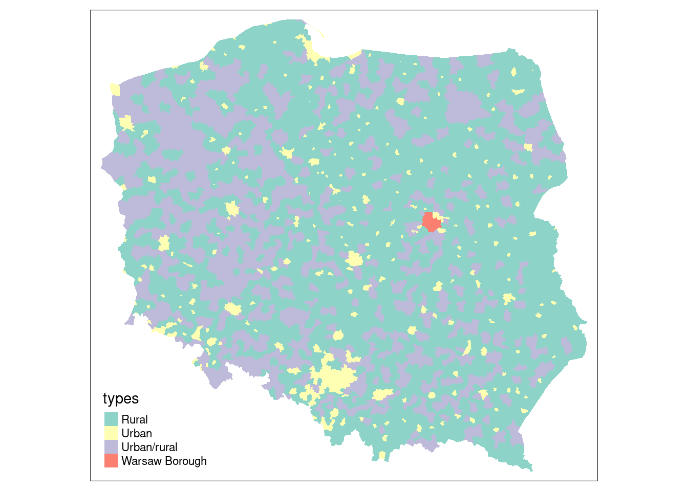
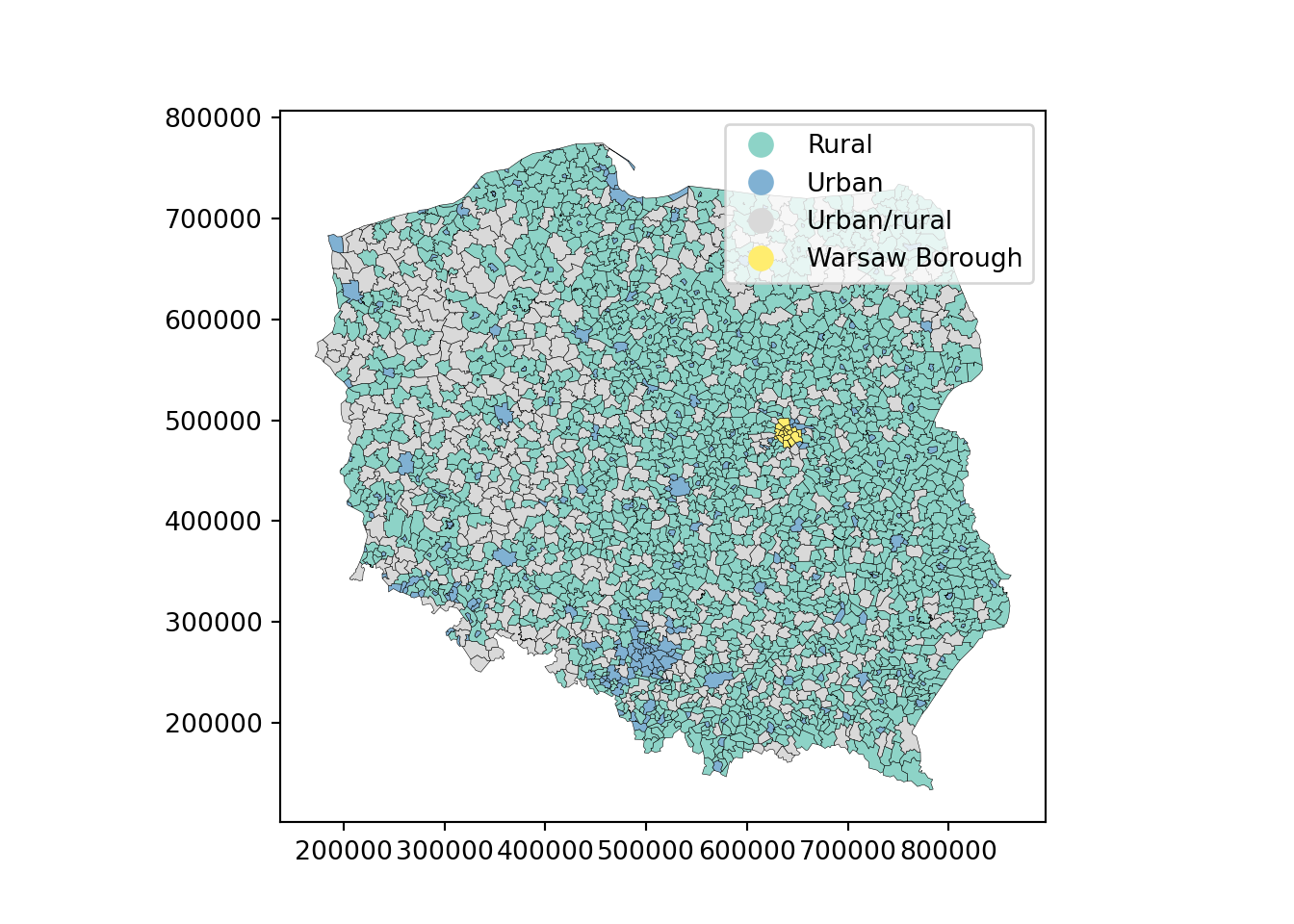
We will be using election data from the 2015 Polish presidential election in this chapter, with 2495 municipalities and Warsaw boroughs (see @fig-plotpolpres15) for a **tmap** map (@sec-tmap) of the municipality types, and complete count data from polling stations aggregated to these areal units. The data are an **sf** `sf` object:
\index{Polish Presidential election data}
\index{tmap}
\index{spDataLarge}
```{r setup_sa0, include=FALSE}
knitr::opts_chunk$set(echo = TRUE, paged.print=FALSE)
owidth <- getOption("width")
xargs <- function(x) {
o <- capture.output(args(x))
oo <- gsub(" *", " ", paste(o[-length(o)], collapse=""))
ooo <- strwrap(oo, width=getOption("width"), indent=1, exdent=3)
cat(paste(ooo, collapse="\n"), "\n")
}
library(tmap, warn.conflicts = FALSE)
tmap4 <- packageVersion("tmap") >= "3.99"
```
::: panel-tabset
#### R
```{r fig-plotpolpres15}
library(sf)
data(pol_pres15, package = "spDataLarge")
pol_pres15 |>
subset(select = c(TERYT, name, types)) |>
head()
#| out.width: 100%
#| fig.cap: "Polish municipality types 2015"
if (tmap4) {
tm_shape(pol_pres15) +
tm_fill("types", fill.scale = tm_scale(values = "brewer.set3"),
fill.legend = tm_legend(position = tm_pos_in("left", "bottom"),
frame.lwd=0, item.r = 0)
)
} else {
tm_shape(pol_pres15) + tm_fill("types")
}
```
#### Python
```{python}
import matplotlib.pyplot as plt
import geopandas as gpd
url = "data/pol_pres15.geojson"
gdf = gpd.read_file(url)
df_subset = gdf[["TERYT", "name", "types"]].head()
print(df_subset)
cmap = "Set3"
ax = gdf.plot(
column="types",
cmap=cmap,
legend=True,
edgecolor="black",
linewidth=0.2,
)
plt.show()
```
:::
For safety's sake, we impose topological validity
::: panel-tabset
#### R
```{r}
if (!all(st_is_valid(pol_pres15)))
        pol_pres15 <- st_make_valid(pol_pres15)
```
#### Python
```{python}
from shapely.validation import make_valid


if not gdf.is_valid.all():
    # Apply make_valid to each geometry
    gdf['geometry'] = gdf['geometry'].apply(make_valid)
```
:::
\index[function]{st\_make\_valid}
Between early 2002 and April 2019, **spdep** contained functions for constructing and handling neighbour and spatial weights objects, tests for spatial autocorrelation, and model fitting functions. The latter have been split out into **spatialreg**, and will be discussed in subsequent chapters. **spdep** [@R-spdep] now accommodates objects represented using **sf** classes and **sp** classes directly.
\index{spatialreg}
\index{spdep}
::: panel-tabset
#### R
```{r, message=FALSE}
library(spdep) |> suppressPackageStartupMessages()
```
#### Python
```{python}
import libpysal
## In python the libpysal library has modules libpysal.graph and libpysal.weights that are equivalent to the spdep
print(f"libpysal version: {libpysal.__version__}")
```
:::
## Contiguous neighbours
\index{neighbours!contiguous}
\index{contiguous neighbours}
\index[function]{poly2nb}
The `poly2nb` function in **spdep** takes the boundary points making up the polygon boundaries in the object passed as the `pl` argument, typically an `"sf"` or `"sfc"` object with `"POLYGON"` or `"MULTIPOLYGON"` geometries. For each observation, the function checks whether at least one (`queen=TRUE`, default), or at least two (rook, `queen=FALSE`) points are within `snap` distance units of each other. The distances are planar in the raw coordinate units, ignoring geographical projections. Once the required number of sufficiently close points is found, the search is stopped.
::: panel-tabset
#### R
```{r, echo=TRUE, eval=FALSE}
args(poly2nb)
```
#### Python
```{python}
# equivalent to poly2nb, libpysal creates the spatial neighbours using method graph.Graph.build_contiguity(gdf) from graph module
# and this method takes in geometry which can be in form of geodataframes
from libpysal import graph
import inspect
print(inspect.signature(graph.Graph.build_contiguity))
```
:::
```{r, echo=FALSE, eval=TRUE}
xargs(poly2nb)
```
From **spdep** 1.1-7, the **sf** package GEOS interface is used within `poly2nb` to find the candidate neighbours and populate `foundInBox` internally. In this case, the use of spatial indexing (STRtree queries) in GEOS through **sf** is the default:
::: panel-tabset
#### R
```{r}
pol_pres15 |> poly2nb(queen = TRUE) -> nb_q
```
#### Python
```{python}
from libpysal import graph

nb_q = graph.Graph.build_contiguity(gdf, rook=False)
## here rook is TRUE by defualt and to use queen based contiguity method set rook = FALSE
```
:::
The print method shows the summary structure of the neighbour object:
::: panel-tabset
#### R
```{r}
nb_q
```
#### Python
```{python}
##recreating the description of neibhorhood/weights exactly as R
summary = nb_q.summary()
print(summary)
```
:::
From **sf** version 1.0-0, the **s2** package [@R-s2] is used by default for spherical geometries, as `st_intersects` used in `poly2nb` passes calculation to `s2::s2_intersects_matrix` (see @sec-spherical). From **spdep** version 1.1-9, if `sf_use_s2()` is `TRUE`, spherical intersection is used to find candidate neighbours; as with GEOS, the underlying `s2` library uses fast spatial indexing.
```{r}
old_use_s2 <- sf_use_s2()
```
\index[function]{sf\_use\_s2}
```{r}
sf_use_s2(TRUE)
```
```{r}
(pol_pres15 |> st_transform("OGC:CRS84") -> pol_pres15_ll) |>
    poly2nb(queen = TRUE) -> nb_q_s2
```
\index{queen neighbours}
\index{neighbours!queen}
Spherical and planar intersection of the input polygons yield the same contiguity neighbours in this case; in both cases valid input geometries are desirable:
```{r}
all.equal(nb_q, nb_q_s2, check.attributes=FALSE)
```
Note that `nb` objects record both symmetric neighbour relationships `i` to `j` and `j` to `i`, because these objects admit asymmetric relationships as well, but these duplications are not needed for object construction.
Most of the **spdep** functions for constructing neighbour objects take a `row.names` argument, the value of which is stored as a `region.id` attribute. If not given, the values are taken from `row.names()` of the first argument. These can be used to check that the neighbours object is in the same order as data. If `nb` objects are subsetted, the indices change to continue to be within `1:length(subsetted_nb)`, but the `region.id` attribute values point back to the object from which it was constructed. This is used in out-of-sample prediction from spatial regression models discussed briefly in @sec-spateconpred.
We can also check that this undirected graph is connected using the `n.comp.nb` function; while some model estimation techniques do not support graphs that are not connected, it is helpful to be aware of possible problems [@FRENISTERRANTINO201825]:
```{r}
(nb_q |> n.comp.nb())$nc
```
\index[function]{n.comp.nb}
This approach is equivalent to treating the neighbour object as a graph and using graph analysis on that graph [@csardi+nepusz:06; @R-igraph], by first coercing to a binary sparse matrix [@R-Matrix]:
::: panel-tabset
#### R
```{r}
library(Matrix, warn.conflicts = FALSE)
library(spatialreg, warn.conflicts = FALSE)
nb_q |>
nb2listw(style = "B") |>
as("CsparseMatrix") -> smat
library(igraph, warn.conflicts = FALSE)
(smat |> graph_from_adjacency_matrix() -> g1) |>
count_components()
```
#### Python
```{python}
import networkx as nx
## using networkx library to convert libpysal Graph object to a NetworkX graph.
w_q = nb_q.to_W()
g1 = w_q.to_networkx()
#Ensuring symmetric
g1 = g1.to_undirected()
# connected components
print(nx.number_connected_components(g1))
```
:::
\index[function]{nb2listw}
\index[function]{graph\_from\_adjacency\_matrix}
\index[function]{count\_components}
Neighbour objects may be exported and imported in GAL format for exchange with other software, using `write.nb.gal` and `read.gal`:
```{r}
tf <- tempfile(fileext = ".gal")
write.nb.gal(nb_q, tf)
```
\index[function]{write.nb.gal}
## Graph-based neighbours
If areal units are an appropriate representation, but only points on the plane have been observed, contiguity relationships may be approximated using graph-based neighbours. In this case, the imputed boundaries tessellate the plane such that points closer to one observation than any other fall within its polygon. The simplest form is by using triangulation, here using the `deldir` function in the **deldir** package. Because the function returns from $i$ and to $j$ identifiers, it is easy to construct a long representation of a `listw` object, as used in the S-Plus SpatialStats module and the `sn2listw` function internally to construct an `nb` object (ragged wide representation). Alternatives such as GEOS often fail to return sufficient information to permit the neighbours to be identified.
The output of these functions is then converted to the `nb` representation using `graph2nb`, with the possible use of the `sym` argument to coerce to symmetry. We take the centroids of the largest component polygon for each observation as the point representation; population-weighted centroids might have been a better choice if they were available:
::: panel-tabset
#### R
```{r}
pol_pres15 |>
st_geometry() |>
st_centroid(of_largest_polygon = TRUE) -> coords
(coords |> tri2nb() -> nb_tri)
```
#### Python
```{python}
# libpysal has a module Delaunay which constructs the Delaunay graph
# from a geo-dataframe consisting input points
from libpysal import weights
import numpy as np
gdf_points = gdf.copy()
gdf_points["geometry"] = gdf_points.centroid
# Delaunay weights (W object)
w_delaunay = weights.Delaunay.from_dataframe(gdf_points)
coords = np.column_stack(
[gdf_points.geometry.x.to_numpy(), gdf_points.geometry.y.to_numpy()]
)
```
:::
\index[function]{tri2nb}
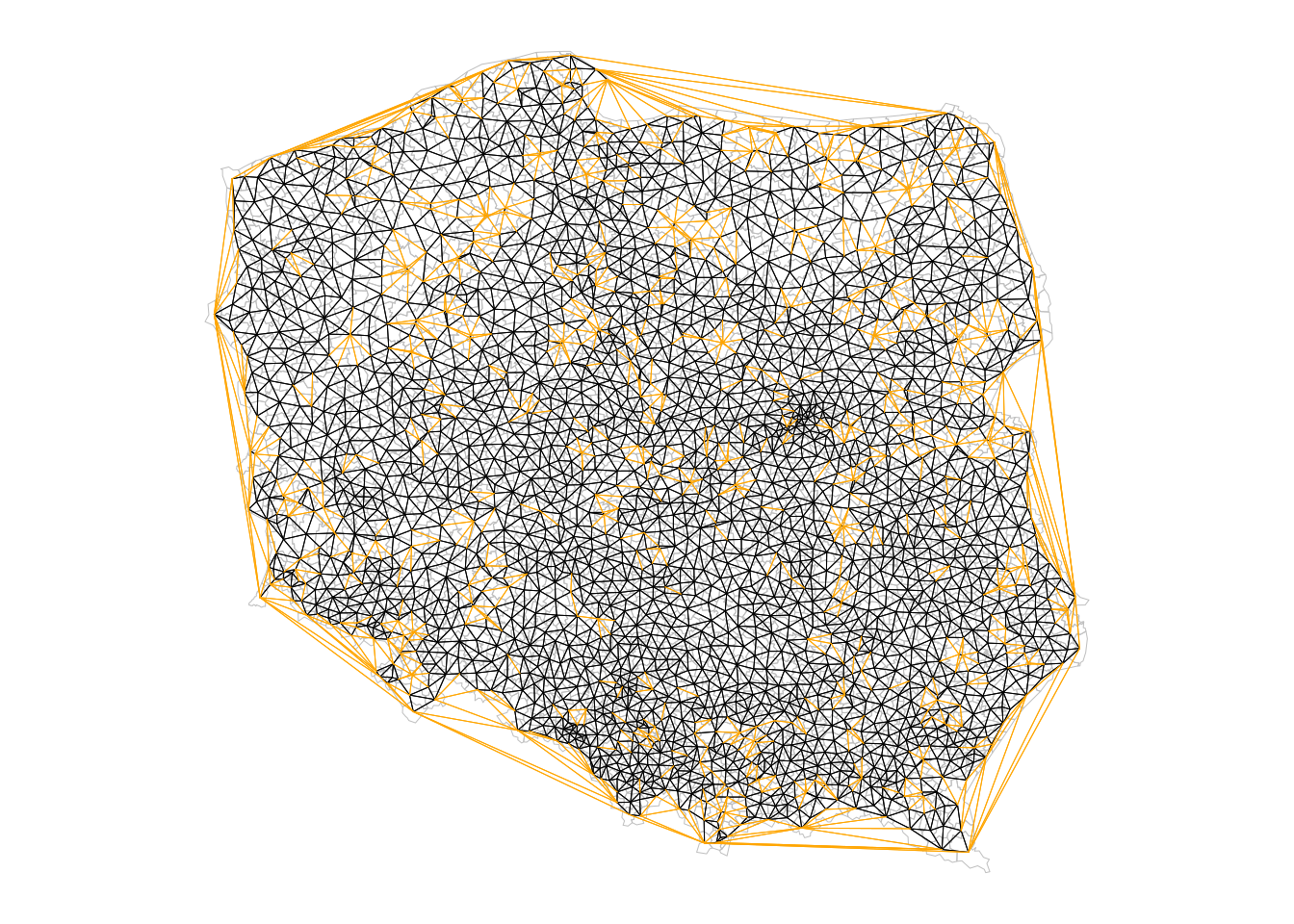
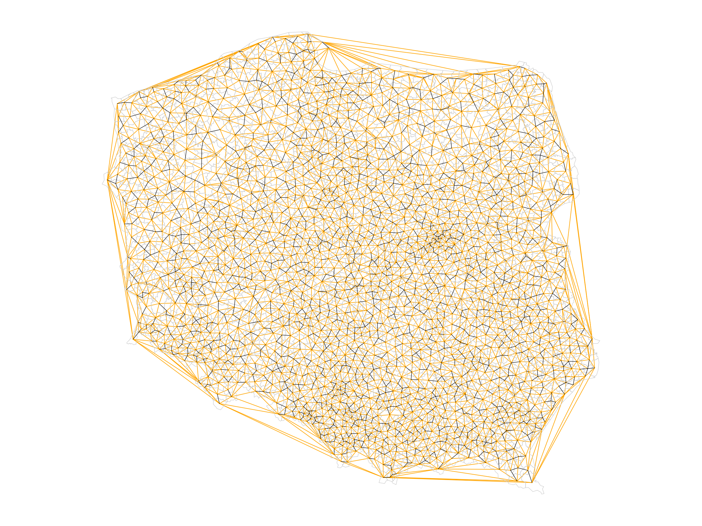
The average number of neighbours is similar to the Queen boundary contiguity case, but if we look at the distribution of edge lengths using `nbdists()`, we can see that although the upper quartile is about 15 km, the maximum is almost 300 km, an edge along much of one side of the convex hull. The short minimum distance is also of interest, as many centroids of urban municipalities are very close to the centroids of their surrounding rural counterparts.
\index{neighbours!edge lengths}
\index[function]{nbdists}
::: panel-tabset
#### R
```{r}
nb_tri |>
nbdists(coords) |>
unlist() |>
summary()
```
#### Python
```{python}
# Extract neighbor pairs (edges)
edge_lengths = []
for i, nbs in w_delaunay.neighbors.items():
for j in nbs:
if i < j:
edge_lengths.append(np.linalg.norm(coords[i] - coords[j]))
edge_lengths = np.array(edge_lengths)
print("Edge length summary:")
print("min:", np.min(edge_lengths))
print("25%:", np.percentile(edge_lengths, 25))
print("median:", np.median(edge_lengths))
print("75%:", np.percentile(edge_lengths, 75))
print("max:", np.max(edge_lengths))
print("mean:", np.mean(edge_lengths))
```
:::
Triangulated neighbours also yield a connected graph:
::: panel-tabset
#### R
```{r}
(nb_tri |> n.comp.nb())$nc
```
#### Python
```{python}
import numpy as np
labels = w_delaunay.component_labels
n_components = len(np.unique(labels))
print("Number of connected components (Delaunay):", n_components)
```
:::
\index[function]{n.comp.nb}
Graph-based approaches include `soi.graph` - discussed here, `relativeneigh` and `gabrielneigh`.
The Sphere of Influence `soi.graph` function takes triangulated neighbours and prunes off neighbour relationships represented by edges that are unusually long for each point, especially around the convex hull [@avis+horton:1985].
```{r}
(nb_tri |>
soi.graph(coords) |>
graph2nb() -> nb_soi)
```
Unpicking the triangulated neighbours does however remove the connected character of the underlying graph:
\index{neighbours!sphere of influence}
\index{sphere of influence}
\index[function]{soi.graph}
\index[function]{relativeneigh}
\index[function]{gabrielneigh}
::: panel-tabset
#### R
```{r}
(nb_soi |> n.comp.nb() -> n_comp)$nc
```
#### Python
```{python}
## unable to produce same result as the R code
import numpy as np
from scipy.spatial import KDTree
import networkx as nx
import matplotlib.pyplot as plt
# coords is Nx2 array of centroid coordinates
# Find nearest neighbor distance for each point
kdt = KDTree(coords)
dists, _ = kdt.query(coords, k=2) # k=2: self + nearest neighbor
nearest = dists[:, 1]
# Build Sphere of Influence (SOI) neighbors:
# Create dict: for each point, neighbors are Delaunay neighbors
# whose edge length <= either point's nearest neighbor distance
soi_neighbors = {i: [] for i in range(len(coords))}
for i, neighbors in w_delaunay.neighbors.items():
for j in neighbors:
if i < j:
dist_ij = np.linalg.norm(coords[i] - coords[j])
if dist_ij <= nearest[i] or dist_ij <= nearest[j]:
soi_neighbors[i].append(j)
soi_neighbors[j].append(i)
# Convert to NetworkX graph
G_soi = nx.Graph()
G_soi.add_nodes_from(range(len(coords)))
for i, ns in soi_neighbors.items():
for j in ns:
if i < j:
G_soi.add_edge(i, j)
# Connected components info
components_soi = list(nx.connected_components(G_soi))
print("Number of connected components (SOI):", len(components_soi))
```
:::
The algorithm has stripped out longer edges leading to urban and rural municipality pairs where their centroids are very close to each other because the rural ones completely surround the urban, giving 15 pairs of neighbours unconnected to the main graph:
```{r}
table(n_comp$comp.id)
```
The largest length edges along the convex hull have been removed, but "holes" have appeared where the unconnected pairs of neighbours have appeared. The differences between `nb_tri` and `nb_soi` are shown in orange in @fig-plotnbdiff.
::: panel-tabset
#### R
```{r fig-plotnbdiff, echo=!knitr::is_latex_output()}
#| fig.cap: "Triangulated (orange + black) and sphere of influence neighbours (black); apparent holes appear for sphere of influence neighbours where an urban municipality is surrounded by a dominant rural municipality (see @fig-plotpolpres15)"
#| code-fold: true
#| out.width: 100%
opar <- par(mar = c(0,0,0,0)+0.5)
pol_pres15 |>
st_geometry() |>
plot(border = "grey", lwd = 0.5)
nb_soi |> plot(coords = coords, add = TRUE,
points = FALSE, lwd = 0.5)
nb_tri |>
diffnb(nb_soi) |>
plot(coords = coords, col = "orange", add = TRUE,
points = FALSE, lwd = 0.5)
par(opar)
```
#### Python
```{python}
import matplotlib.pyplot as plt
fig, ax = plt.subplots(figsize=(12, 9))
# Plot polygon outlines in light gray (no fill)
gdf.boundary.plot(ax=ax, color="#cccccc", linewidth=0.5)
# SOI edges: black, thin
drawn_soi = set()
for i, nbs in soi_neighbors.items():
for j in nbs:
if i < j and (i, j) not in drawn_soi:
ax.plot(
[coords[i][0], coords[j][0]],
[coords[i][1], coords[j][1]],
color="black",
linewidth=0.5,
zorder=2
)
drawn_soi.add((i, j))
# Delaunay minus SOI: orange, thin
drawn_dif = set()
for i, nbs in w_delaunay.neighbors.items():
for j in nbs:
if i < j and (i, j) not in drawn_soi and (i, j) not in drawn_dif:
ax.plot(
[coords[i][0], coords[j][0]],
[coords[i][1], coords[j][1]],
color="orange",
linewidth=0.7,
zorder=1
)
drawn_dif.add((i, j))
# Centroids: tiny dots, on top
# ax.scatter(coords[:, 0], coords[:, 1], color="black", s=8, zorder=3)
ax.set_aspect("equal")
ax.set_axis_off()
plt.tight_layout()
plt.show()
```
:::
## Distance-based neighbours
\index{neighbours!distance-based}
\index{distance-based neighbours}
\index[function]{dnearneigh}
Distance-based neighbours can be constructed using `dnearneigh`, with a distance band with lower `d1` and upper `d2` bounds controlled by the `bounds` argument. If spherical coordinates are used and either specified in the coordinates object `x` or with `x` as a two-column matrix and `longlat=TRUE`, great circle distances in kilometre will be calculated assuming the WGS84 reference ellipsoid, or if `use_s2=TRUE` (the default value) using the spheroid (see @sec-spherical). If `dwithin` is `FALSE` and the version of **s2** is greater than `1.0.7`, `s2_closest_edges` may be used, if `TRUE` and `use_s2=TRUE`, `s2_dwithin_matrix` is used; both of these methods use fast spherical spatial indexing, but because `s2_closest_edges` takes minimum and maximum bounds, it only needs one pass in the R code of `dnearneigh`.
\index[function]{s2\_closest\_edges}
Arguments have been added to use functionality in the **dbscan** package [@R-dbscan] for finding neighbours using planar spatial indexing in two or three dimensions by default, and not to test the symmetry of the output neighbour object. In addition, three arguments relate to the use of spherical geometry distance measurements.
\index{neighbours!k nearest}
\index{nearest neighbours}
\index[function]{knearneigh}
\index[function]{knn2nb}
The `knearneigh` function for $k$-nearest neighbours returns a `knn` object, converted to an `nb` object using `knn2nb`. It can also use great circle distances, not least because nearest neighbours may differ when unprojected coordinates are treated as planar. `k` should be a small number. For projected coordinates, the **dbscan** package is used to compute nearest neighbours more efficiently. Note that `nb` objects constructed in this way are most unlikely to be symmetric hence `knn2nb` has a `sym` argument to permit the imposition of symmetry, which will mean that all units have at least `k` neighbours, not that all units will have exactly `k` neighbours. When `sf_use_s2()` is `TRUE`, `knearneigh` will use fast spherical spatial indexing when the input object is of class `"sf"` or `"sfc"`.
\index[function]{nbdists}
The `nbdists` function returns the length of neighbour relationship edges in the units of the coordinates if the coordinates are projected, in kilometre otherwise. In order to set the upper limit for distance bands, one may first find the maximum first nearest neighbour distance, using `unlist` to remove the list structure of the returned object. When `sf_use_s2()` is `TRUE`, `nbdists` will use fast spherical distance calculations when the input object is of class `"sf"` or `"sfc"`.
::: panel-tabset
#### R
```{r}
coords |>
knearneigh(k = 1) |>
knn2nb() |>
nbdists(coords) |>
unlist() |>
summary()
```
#### Python
```{python}
# 1-nearest neighbour graph (k = 1)
knn1 = graph.Graph.build_knn(coords, k=1)
# distances of neighbour relationships
# knn1.to_W().neighbors is a dict: i -> list of neighbours
# compute edge lengths using coords
dists = []
for i, nbs in knn1.to_W().neighbors.items():
for j in nbs:
if i < j: # count each edge once
d = np.linalg.norm(coords[i] - coords[j])
dists.append(d)
dists = np.array(dists)
print("Min:", np.min(dists))
print("1st Qu.:", np.percentile(dists, 25))
print("Median:", np.median(dists))
print("Mean:", np.mean(dists))
print("3rd Qu.:", np.percentile(dists, 75))
print("Max:", np.max(dists))
```
:::
Here the largest first nearest neighbour distance is just under 18 km, so using this as the upper threshold gives certainty that all units will have at least one neighbour:
::: panel-tabset
#### R
```{r}
coords |> dnearneigh(0, 18000) -> nb_d18
```
#### Python
```{python}
nb_d18 = graph.Graph.build_distance_band(
    coords,
    threshold=18000,
    binary=True  # match spdep: 1 if within band, 0 otherwise
)
```
:::
For this moderate number of observations, use of spatial indexing does not yield advantages in run times:
-
::: panel-tabset
#### R
```{r}
coords |> dnearneigh(0, 18000, use_kd_tree = FALSE) -> nb_d18a
```
#### Python
```{python}
# In libpysal’s Graph.build_distance_band, the efficient search/indexing strategy is internal and not user‑switchable, so Python only constructs the object once and does not need an explicit equality check.
```
:::
and the output objects are the same:
```{r}
all.equal(nb_d18, nb_d18a, check.attributes = FALSE)
```
::: panel-tabset
#### R
```{r}
nb_d18
```
#### Python
```{python}
nb_d18.summary()
```
:::
However, even though there are no no-neighbour observations (their presence is reported by the print method for `nb` objects), the graph is not connected, as a pair of observations are each others' only neighbours.
::: panel-tabset
#### R
```{r}
(nb_d18 |> n.comp.nb() -> n_comp)$nc
```
#### Python
```{python}
print("Number of connected components:", nb_d18.n_components)
```
:::
```{r}
table(n_comp$comp.id)
```
Adding 300 m to the threshold gives us a neighbour object with no no-neighbour units, and all units can be reached from all others across the graph.
::: panel-tabset
#### R
```{r}
(coords |> dnearneigh(0, 18300) -> nb_d183)
```
#### Python
```{python}
nb_d183 = graph.Graph.build_distance_band(
    coords,
    threshold=18300,
    binary=True
)
```
:::
::: panel-tabset
#### R
```{r}
(nb_d183 |> n.comp.nb())$nc
```
#### Python
```{python}
print("Number of connected components (18.3 km):", nb_d183.n_components)
```
:::
One characteristic of distance-based neighbours is that more densely settled areas, with units which are smaller in terms of area, have higher neighbour counts (Warsaw boroughs are much smaller on average, but have almost 30 neighbours for this distance criterion). Having many neighbours smooths the neighbour relationship across more neighbours.
For use later, we also construct a neighbour object with no-neighbour units, using a threshold of 16 km:
::: panel-tabset
#### R
```{r}
(coords |> dnearneigh(0, 16000) -> nb_d16)
```
#### Python
```{python}
nb_d16 = graph.Graph.build_distance_band(
coords,
threshold=16000,
binary=True
)
# number of isolates (no-neighbour units)
isolates_16 = nb_d16.isolates
print("Number of isolates (16 km):", len(isolates_16))
```
:::
It is possible to control the numbers of neighbours directly using $k$-nearest neighbours, either accepting asymmetric neighbours:
::: panel-tabset
#### R
```{r}
((coords |> knearneigh(k = 6) -> knn_k6) |> knn2nb() -> nb_k6)
```
#### Python
```{python}
nb_k6 = graph.Graph.build_knn(
    coords,
    k=6
)
```
:::
or imposing symmetry:
::: panel-tabset
#### R
```{r}
(knn_k6 |> knn2nb(sym = TRUE) -> nb_k6s)
```
#### Python
```{python}
## no inbuilt function in libpysal to enforce the symmetry

# Asymmetric k-NN (k = 6)
nb_k6 = graph.Graph.build_knn(coords, k=6)

# Convert to W
w_k6 = nb_k6.to_W()

# Symmetrise the neighbours:
#    create the union of i->j and j->i, then set binary weights
sym_neighbors = {}
for i, nbs in w_k6.neighbors.items():
    sym_neighbors.setdefault(i, set()).update(nbs)
    for j in nbs:
        sym_neighbors.setdefault(j, set()).add(i)

# Build a symmetric W from the symmetrised neighbor dict

sym_neighbors_dict = {i: list(js) for i, js in sym_neighbors.items()}
w_k6s = weights.W(sym_neighbors_dict)

# Convert back to Graph
nb_k6s = graph.Graph.from_W(w_k6s)
```
Here the size of `k` is sufficient to ensure connectedness, although the graph is not planar as edges cross at locations other than nodes, which is not the case for contiguous or graph-based neighbours.
::: panel-tabset
#### R
```{r}
(nb_k6s |> n.comp.nb())$nc
```
#### Python
```{python}
print(nb_k6s.n_components)
```
:::
In the case of points on the sphere (see @sec-spherical), the output of `st_centroid` will differ, so rather than inverse projecting the points, we extract points as geographical coordinates from the inverse projected polygon geometries:
```{r}
old_use_s2 <- sf_use_s2()
```
```{r}
sf_use_s2(TRUE)
```
::: panel-tabset
#### R
```{r}
pol_pres15_ll |>
    st_geometry() |>
    st_centroid(of_largest_polygon = TRUE) -> coords_ll
```
#### Python
```{python}
# convert the projection of the polygons to geographic CRS (WGS84)
from pyproj import CRS
# Initialize CRS using the OGC URN string
crs_ogc_84 = CRS("OGC:CRS84")
gdf_ll = gdf.to_crs(crs_ogc_84)
# Centroids
gdf_ll_centroids = gdf_ll.copy()
gdf_ll_centroids["geometry"] = gdf_ll_centroids.geometry.centroid
coords_ll = np.column_stack(
[gdf_ll_centroids.geometry.x.to_numpy(),
gdf_ll_centroids.geometry.y.to_numpy()]
)
```
:::
For spherical coordinates, distance bounds are in kilometres:
::: panel-tabset
#### R
```{r}
(coords_ll |> dnearneigh(0, 18.3, use_s2 = TRUE,
dwithin = TRUE) -> nb_d183_ll)
```
#### Python
```{python}
# Convert degrees to radians for haversine
coords_ll_rad = np.radians(coords_ll)
def haversine_rad(p, q, R=6371.0):
lon1, lat1 = p
lon2, lat2 = q
dlon = lon2 - lon1
dlat = lat2 - lat1
a = (
np.sin(dlat / 2.0) ** 2
+ np.cos(lat1) * np.cos(lat2) * np.sin(dlon / 2.0) ** 2
)
c = 2 * np.arcsin(np.sqrt(a))
return R * c # distance in km
max_dist_km = 18.3
n = coords_ll_rad.shape[0]
neighbors_sph = {i: [] for i in range(n)}
for i in range(n):
for j in range(i + 1, n):
d_ij = haversine_rad(coords_ll_rad[i], coords_ll_rad[j])
if 0 < d_ij <= max_dist_km:
neighbors_sph[i].append(j)
neighbors_sph[j].append(i)
# build graph from neighbour's distances from_dicts
nb_d183_ll = graph.Graph.from_dicts(neighbors_sph, weights = None)
print(nb_d183_ll.summary())
```
:::
These neighbours differ from the spherical 18.3 km neighbours as would be expected:
::: panel-tabset
#### R
```{r}
isTRUE(all.equal(nb_d183, nb_d183_ll, check.attributes = FALSE))
```
#### Python
```{python}
print(nb_d183 == nb_d183_ll)
```
:::
If **s2** providing faster distance neighbour indexing is available, by default `s2_closest_edges` will be used for geographical coordinates:
```{r}
(coords_ll |> dnearneigh(0, 18.3) -> nb_d183_llce)
```
where the two **s2**-based neighbour objects are the same:
```{r}
isTRUE(all.equal(nb_d183_llce, nb_d183_ll,
check.attributes = FALSE))
```
Fast spherical spatial indexing in **s2** is used to find $k$ nearest neighbours:
-
::: panel-tabset
#### R
```{r}
(coords_ll |> knearneigh(k = 6) |> knn2nb() -> nb_k6_ll)
```
#### Python
```{python}
# The 'haversine' metric in Python typically requires inputs in radians.
coords_ll_rad = np.radians(coords_ll)

nb_k6_ll = graph.Graph.build_knn(
    coords_ll_rad,
    k=6,
    metric="haversine"
) ##needs scikit installed
```
:::
These neighbours differ from the planar `k=6` nearest neighbours as would be expected, but will also differ slightly from legacy brute-force ellipsoid distances:
```{r}
isTRUE(all.equal(nb_k6, nb_k6_ll, check.attributes = FALSE))
```
The `nbdists` function also uses **s2** to find distances on the sphere when the `"sf"` or `"sfc"`input object is in geographical coordinates (distances returned in kilometres):
```{r}
nb_q |> nbdists(coords_ll) |> unlist() |> summary()
```
These differ a little for the same weights object when planar coordinates are used (distances returned in the metric of the points for planar geometries and kilometres for ellipsoidal and spherical geometries):
```{r}
nb_q |> nbdists(coords) |> unlist() |> summary()
```
```{r, results='hide'}
sf_use_s2(old_use_s2)
```
## Weights specification
Once neighbour objects are available, further choices need to be made in specifying the weights objects. The `nb2listw` function is used to create a `listw` weights object with an `nb` object, a matching list of weights vectors, and a style specification. Because handling no-neighbour observations now begins to matter, the `zero.policy` argument is introduced. By default, this is `FALSE`, indicating that no-neighbour observations will cause an error, as the spatially lagged value for an observation with no neighbours is not available. By convention, zero is substituted for the lagged value, as the cross-product of a vector of zero-valued weights and a data vector, hence the name of `zero.policy`.
\index[function]{nb2listw}
\index{weights!objects}
\index{weights!listw}
```{r, echo=TRUE, eval=FALSE}
args(nb2listw)
```
```{r, echo=FALSE, eval=TRUE}
xargs(nb2listw)
```
We will be using the helper function `spweights.constants` below to show some consequences of varying style choices. It returns constants for a `listw` object, $n$ is the number of observations, `n1` to `n3` are $n-1, \ldots$, `nn` is $n^2$ and $S_0$, $S_1$ and $S_2$ are constants, $S_0$ being the sum of the weights. There is a full discussion of the constants in @Bivand2018.
\index[function]{spweights.constants}
```{r, echo=TRUE, eval=FALSE}
args(spweights.constants)
```
```{r, echo=FALSE, eval=TRUE}
xargs(spweights.constants)
```
The `"B"` binary style gives a weight of unity to each neighbour relationship, and typically up-weights units with no boundaries on the edge of the study area, having a higher count of neighbours.
::: panel-tabset
#### R
```{r}
(nb_q |>
nb2listw(style = "B") -> lw_q_B) |>
spweights.constants() |>
data.frame() |>
subset(select = c(n, S0, S1, S2))
```
#### Python
```{python}
import pandas as pd
# In libpysal, we convert the Graph (nb_q) to a W object to handle weights and styles.
# style='B' in spdep is Binary.
# nb_q.to_W() creates a W object. By default, weights are binary.
w_q_B = nb_q.to_W()
# Ensure it is not standardized (though default is usually unstandardized)
w_q_B.transform = 'b' # 'b' for binary (explicitly)
# libpysal W objects have properties for the constants S0, S1, S2
constants_B = pd.DataFrame({
'n': [w_q_B.n],
'S0': [w_q_B.s0],
'S1': [w_q_B.s1],
'S2': [w_q_B.s2]
})
print(constants_B)
```
\index{weights!row-standardised}
The `"W"` row-standardised style up-weights units around the edge of the study area that necessarily have fewer neighbours. This style first gives a weight of unity to each neighbour relationship, then it divides these weights by the per unit sums of weights. Naturally this leads to division by zero where there are no neighbours, a not-a-number result, unless the chosen policy is to permit no-neighbour observations. We can see that $S_0$ is now equal to $n$.
::: panel-tabset
#### R
```{r}
(nb_q |>
nb2listw(style = "W") -> lw_q_W) |>
spweights.constants() |>
data.frame() |>
subset(select = c(n, S0, S1, S2))
```
#### Python
```{python}
# Create row-standardised weights (style="W" equivalent is transform='r')
w_q_W = nb_q.to_W()
w_q_W.transform = 'r'
constants_W = pd.DataFrame({
'n': [w_q_W.n],
'S0': [w_q_W.s0],
'S1': [w_q_W.s1],
'S2': [w_q_W.s2]
})
print(constants_W)
```
:::
\index{weights!inverse distance}
Inverse distance weights are used in a number of scientific fields. Some use dense inverse distance matrices, but many of the inverse distances are close to zero, have little practical contribution, especially as the spatial process matrix is itself dense. Inverse distance weights may be constructed by taking the lengths of edges, changing units to avoid most weights being too large or small (here from metre to kilometre), taking the inverse, and passing through the `glist` argument to `nb2listw`:
::: panel-tabset
#### R
```{r}
nb_d183 |>
nbdists(coords) |>
lapply(function(x) 1/(x/1000)) -> gwts
(nb_d183 |> nb2listw(glist=gwts, style="B") -> lw_d183_idw_B) |>
spweights.constants() |>
data.frame() |>
subset(select=c(n, S0, S1, S2))
```
#### Python
```{python}
import numpy as np
from libpysal import weights
# Calculate custom Inverse Distance Weights (1 / distance_in_km)
# reuse the nb_d183 Graph structure created earlier
idw_weights = {}
neighbors = nb_d183.to_W().neighbors
for i, nbs in neighbors.items():
w_i = []
for j in nbs:
# Calculate distance in meters (Euclidean based on coords)
d_m = np.linalg.norm(coords[i] - coords[j])
# Calculate weight: 1 / (distance in km)
# Note:divide by 1000 to convert meters to km
w = 1.0 / (d_m / 1000.0)
w_i.append(w)
idw_weights[i] = w_i
# Create a W object with these custom weights
# style="B" in R (Basic) means use the raw weights without row-standardization.
# In libpysal, the default transform is 'O' (Original), which preserves these values.
w_d183_idw_B = weights.W(neighbors, idw_weights)
# Calculate constants
constants_idw = pd.DataFrame({
'n': [w_d183_idw_B.n],
'S0': [w_d183_idw_B.s0],
'S1': [w_d183_idw_B.s1],
'S2': [w_d183_idw_B.s2]
})
print(constants_idw)
```
No-neighbour handling is by default to prevent the construction of a weights object, making the analyst take a position on how to proceed.
```{r}
try(nb_d16 |> nb2listw(style="B") -> lw_d16_B)
```
```{python}
nb_d16 = graph.Graph.build_distance_band(coords, threshold=16000, binary=True)
# In Python, we check the length of the isolates list to mimic this check.
if len(nb_d16.isolates) > 0:
print(f"Error: Empty neighbour sets found. (Isolates: {len(nb_d16.isolates)})")
else:
w_d16_B = nb_d16.to_W()
```
Use can be made of the `zero.policy` argument to many functions used with `nb` and `listw` objects.
:::
::: panel-tabset
#### R
```{r}
nb_d16 |>
nb2listw(style="B", zero.policy=TRUE) |>
spweights.constants(zero.policy=TRUE) |>
data.frame() |>
subset(select=c(n, S0, S1, S2))
```
#### Python
```{python}
# libpysal allows creating W with islands by default.
w_d16_B = nb_d16.to_W()
# Note: libpysal includes islands in 'n' (total observations)
# 'S0' for binary weights is the count of non-zero links.
constants_d16 = pd.DataFrame({
'n': [w_d16_B.n],
'S0': [w_d16_B.s0],
'S1': [w_d16_B.s1],
'S2': [w_d16_B.s2]
})
print(constants_d16)
```
:::
Note that by default the `adjust.n` argument to `spweights.constants` is set by default to `TRUE`, subtracting the count of no-neighbour observations from the observation count, so $n$ is smaller with possible consequences for inference. The complete count can be retrieved by changing the argument.
## Higher order neighbours
\index{neighbours!higher order}
We recall the characteristics of the neighbour object based on Queen contiguities:
```{r}
nb_q
```
If we wish to create an object showing $i$ to $k$ neighbours, where $i$ is a neighbour of $j$, and $j$ in turn is a neighbour of $k$, so taking two steps on the neighbour graph, we can use `nblag`, which automatically removes $i$ to $i$ self-neighbours:
::: panel-tabset
#### R
```{r}
(nb_q |> nblag(2) -> nb_q2)[[2]]
```
#### Python
```{python}
from libpysal import weights
# 1. Convert Graph to W (if not already done)
w_q = nb_q.to_W()
# 2. Calculate 2nd order neighbours (strictly 2 steps away)
w_q2 = weights.higher_order(w_q, k=2)
# Check summary to compare with R output (number of nonzero links, etc.)
print(f"Neighbour list object:\nNumber of regions: {w_q2.n}")
print(f"Number of nonzero links: {w_q2.s0}")
print(f"Percentage nonzero weights: {(w_q2.s0 / (w_q2.n**2) * 100):.2f}")
print(f"Average number of links: {w_q2.mean_neighbors:.2f}")
```
:::
The `nblag_cumul` function cumulates the list of neighbours for the whole list of lags:
\index[function]{nblag}
\index[function]{nblag\_cumul}
::: panel-tabset
#### R
```{r}
nblag_cumul(nb_q2)
```
#### Python
```{python}
from libpysal.weights import w_union
# Combine lag 1 (w_q) and lag 2 (w_q2)
# w_union returns a new W object containing all links from both inputs
w_cumul = w_union(w_q, w_q2)
print("Cumulative neighbours (Order 1 + Order 2):")
print(f"Number of regions: {w_cumul.n}")
print(f"Number of nonzero links: {w_cumul.s0}")
print(f"Percentage nonzero weights: {(w_cumul.s0 / (w_cumul.n**2) * 100):.2f}")
print(f"Average number of links: {w_cumul.mean_neighbors:.2f}")
```
:::
while the set operation `union.nb` takes two objects, giving here the same outcome:
\index[function]{union.nb}
```{r}
union.nb(nb_q2[[2]], nb_q2[[1]])
```
Returning to the graph representation of the same neighbour object, we can ask how many steps might be needed to traverse the graph:
\index[function]{diameter}
::: panel-tabset
#### R
```{r}
diameter(g1)
```
#### Python
```{python}
# Calculate diameter using NetworkX
d = nx.diameter(g1)
print(f"Diameter: {d}")
```
:::
We step out from each observation across the graph to establish the number of steps needed to reach each other observation by the shortest path (creating an $n \times n$ matrix `sps`), once again finding the same maximum count.
::: panel-tabset
#### R
```{r}
g1 |> distances() -> sps
(sps |> apply(2, max) -> spmax) |> max()
```
#### Python
```{python}
eccentricities = nx.eccentricity(g1)
spmax = pd.Series(eccentricities)
print(f"Max eccentricity (Diameter): {spmax.max()}")
```
:::
\index[function]{distances}
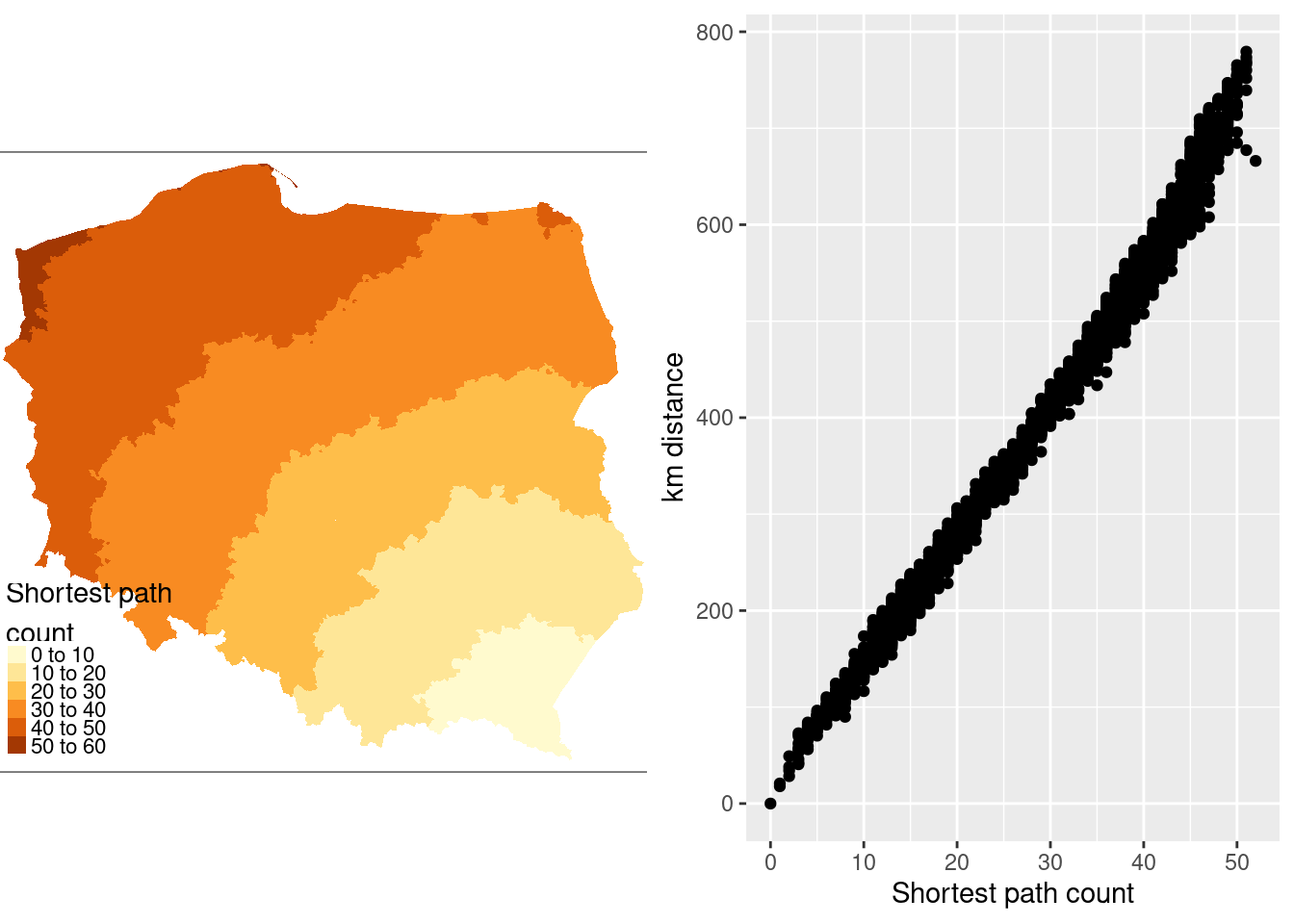
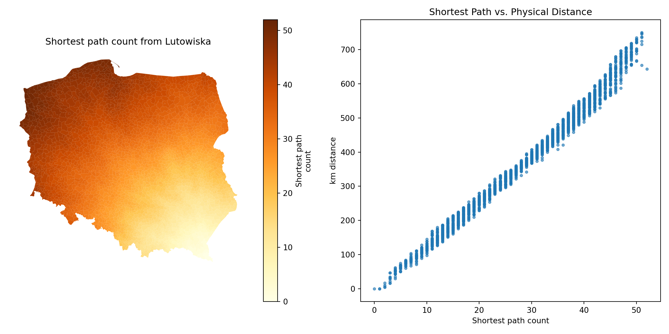
The municipality with the maximum count is called Lutowiska, close to the Ukrainian border in the far south east of the country:
::: panel-tabset
#### R
```{r}
mr <- which.max(spmax)
pol_pres15$name0[mr]
```
#### Python
```{python}
mr = spmax.idxmax()
# Retrieve the name from the GeoDataFrame
remote_municipality = gdf.loc[mr, "name"]
print(f"Most remote municipality: {remote_municipality}")
```
:::
@fig-shortestpath shows that contiguity neighbours represent the same kinds of relationships with other observations as distance. Some approaches prefer distance neighbours on the basis that, for example, inverse distance neighbours show clearly how all observations are related to each other. However, the development of tests for spatial autocorrelation and spatial regression models has involved the inverse of a spatial process model, which in turn can be represented as the sum of a power series of the product of a coefficient and a spatial weights matrix, intrinsically acknowledging the relationships of all observations with all other observations. Sparse contiguity neighbour objects accommodate rich dependency structures without the need to make the structures explicit.
::: panel-tabset
#### R
```{r fig-shortestpath, message=FALSE, echo=!knitr::is_latex_output()}
#| out.width: 100%
#| code-fold: true
#| fig.cap: "Relationship of shortest paths to distance for Lutowiska; left panel: shortest path counts from Lutowiska; right panel: plot of shortest paths from Lutowiska to other observations, and distances from Lutowiska to other observations"
pol_pres15$sps1 <- sps[,mr]
if (!tmap4) {
  tm1 <- tm_shape(pol_pres15) +
          tm_fill("sps1", title = "Shortest path\ncount")
} else {
  tm1 <- tm_shape(pol_pres15) +
      tm_fill("sps1",
          fill.scale = tm_scale(values = "brewer.yl_or_br"),
          fill.legend = tm_legend("Shortest path\ncount", item.r = 0,
              frame = FALSE, position = tm_pos_in("left", "bottom")))
}
coords[mr] |>
    st_distance(coords) |>
    c() |>
    (function(x) x/1000)() |>
    units::set_units(NULL) -> pol_pres15$dist_52
library(ggplot2)
g1 <- ggplot(pol_pres15, aes(x = sps1, y = dist_52)) +
        geom_point() +
        xlab("Shortest path count") +
        ylab("km distance")
gridExtra::grid.arrange(tmap_grob(tm1), g1, nrow=1)
```
#### Python
```{python}
import matplotlib.pyplot as plt
import networkx as nx
path_lengths = nx.single_source_shortest_path_length(g1, source=mr)
# Map these lengths to the GeoDataFrame
gdf['sps1'] = gdf.index.map(path_lengths)
remote_geom = gdf.geometry[mr]
gdf['dist_52'] = gdf.distance(remote_geom) / 1000.0
fig, (ax1, ax2) = plt.subplots(1, 2, figsize=(12, 6))
# Left Panel: Map of Shortest Path Counts
gdf.plot(
column='sps1',
cmap='YlOrBr',
legend=True,
legend_kwds={'label': "Shortest path\ncount"},
ax=ax1
)
ax1.set_axis_off()
ax1.set_title("Shortest path count from Lutowiska")
# Right Panel: Scatter Plot
ax2.scatter(gdf['sps1'], gdf['dist_52'], alpha=0.6, s=10)
ax2.set_xlabel("Shortest path count")
ax2.set_ylabel("km distance")
ax2.set_title("Shortest Path vs. Physical Distance")
plt.tight_layout()
plt.show()
```
:::
```{r echo=FALSE}
save(list = ls(), file = "ch14.RData")
```
```{python echo=FALSE}
import pickle
# save w_q
if 'w_q' not in locals():
w_q = nb_q.to_W()
# Save the necessary variables to a file
with open('ch14_py.pkl', 'wb') as f:
pickle.dump({'gdf': gdf, 'w_q': w_q, 'w_q_B': w_q_B, 'w_d183_idw_B': w_d183_idw_B}, f)
```
## Exercises
1. Which kinds of geometry support are appropriate for which functions creating neighbour objects?
2. Which functions creating neighbour objects are only appropriate for planar representations?
3. What difference might the choice of `rook` rather than `queen` contiguities make on a chessboard?
4. What are the relationships between neighbour set cardinalities (neighbour counts) and row-standardised weights, and how do they open analyses up to edge effects? Use the chessboard you constructed in exercise 3 for both `rook` and `queen` neighbours.