# Geometries {#sec-geometries}
\index{geometry!simple feature}
\index{simple feature!definition}
Having learned how we represent coordinates systems, we can define
how geometries can be described using these coordinate systems. This
chapter will explain:
* _simple features_, a standard that describes point, line, and polygon
geometries along with operations on them,
* operations on geometries,
* coverages, functions of space or space-time,
* tesselations, sub-divisions of larger regions into sub-regions, and
* networks.
Geometries on the sphere are discussed in @sec-spherical, rasters and
other rectangular sub-divisions of space or space time are discussed
in @sec-datacube.
## Simple feature geometries {#sec-simplefeatures}
\index{simple feature geometry}
\index{simple feature!geometry}
Simple feature geometries are a way to describe the geometries of
_features_. By _features_ we mean _things_ that have a geometry,
potentially implicitly some time properties, and further _attributes_ that could
include labels describing the thing and/or values quantitatively measuring it.
The main application of simple feature geometries is to describe
geometries in two-dimensional space by points, lines, or polygons. The
"simple" adjective refers to the fact that the line or polygon
geometries are represented by sequences of points connected with
straight lines that do not self-intersect.
_Simple features access_ is a standard [@sfa; @sfa2; @iso] for
describing simple feature geometries. It includes:
\index{simple feature access}
* a class hierarchy
* a set of operations
* binary and text encodings
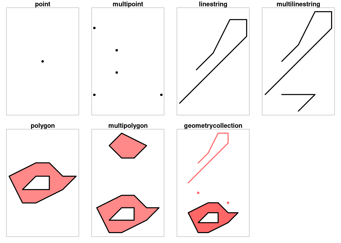
We will first discuss the seven most common simple feature geometry
types.
### The big seven {#sec-seven}
\index{simple feature geometry!types}
\index{POINT}
\index{MULTIPOINT}
\index{LINESTRING}
\index{MULTILINESTRING}
\index{POLYGON}
\index{MULTIPOLYGON}
\index{GEOMETRYCOLLECTION}
The most common simple feature geometries used to represent a _single_ feature are:
| type | description |
|---------------------------|---------------------------------------------------------------------------|
| `POINT` | single point geometry |
| `MULTIPOINT` | set of points |
| `LINESTRING` | single linestring (two or more points connected by straight lines) |
| `MULTILINESTRING` | set of linestrings |
| `POLYGON` | exterior ring with zero or more inner rings, denoting holes |
| `MULTIPOLYGON` | set of polygons |
| `GEOMETRYCOLLECTION` | set of the geometries above |
::: panel-tabset
#### R
```{r fig-sfgeometries, echo=!knitr::is_latex_output(), message = FALSE}
#| fig.cap: "Sketches of the main simple feature geometry types"
#| code-fold: true
library(sf) |> suppressPackageStartupMessages()
par(mfrow = c(2,4))
par(mar = c(1,1,1.2,1))

# 1
p <- st_point(0:1)
plot(p, pch = 16)
title("point")
box(col = 'grey')

# 2
mp <- st_multipoint(rbind(c(1,1), c(2, 2), c(4, 1), c(2, 3), c(1,4)))
plot(mp, pch = 16)
title("multipoint")
box(col = 'grey')

# 3
ls <- st_linestring(rbind(c(1,1), c(5,5), c(5, 6), c(4, 6), c(3, 4), c(2, 3)))
plot(ls, lwd = 2)
title("linestring")
box(col = 'grey')

# 4
mls <- st_multilinestring(list(
  rbind(c(1,1), c(5,5), c(5, 6), c(4, 6), c(3, 4), c(2, 3)),
  rbind(c(3,0), c(4,1), c(2,1))))
plot(mls, lwd = 2)
title("multilinestring")
box(col = 'grey')

# 5 polygon
po <- st_polygon(list(rbind(c(2,1), c(3,1), c(5,2), c(6,3), c(5,3), c(4,4), c(3,4), c(1,3), c(2,1)),
    rbind(c(2,2), c(3,3), c(4,3), c(4,2), c(2,2))))
plot(po, border = 'black', col = '#ff8888', lwd = 2)
title("polygon")
box(col = 'grey')

# 6 multipolygon
mpo <- st_multipolygon(list(
    list(rbind(c(2,1), c(3,1), c(5,2), c(6,3), c(5,3), c(4,4), c(3,4), c(1,3), c(2,1)),
        rbind(c(2,2), c(3,3), c(4,3), c(4,2), c(2,2))),
    list(rbind(c(3,7), c(4,7), c(5,8), c(3,9), c(2,8), c(3,7)))))
plot(mpo, border = 'black', col = '#ff8888', lwd = 2)
title("multipolygon")
box(col = 'grey')

# 7 geometrycollection
gc <- st_geometrycollection(list(po, ls + c(0,5), st_point(c(2,5)), st_point(c(5,4))))
plot(gc, border = 'black', col = '#ff6666', pch = 16, lwd = 2)
title("geometrycollection")
box(col = 'grey')
```
#### Python
```{python}
#| fig.cap: "Sketches of the main simple feature geometry types"
#| code-fold: true
#| eval: true
import matplotlib.pyplot as plt
import geopandas as gpd
from shapely.geometry import Point, MultiPoint, LineString, MultiLineString, Polygon, MultiPolygon

# Set up a 2x4 grid of plots
plt.figure(figsize=(12, 6))
plt.subplots_adjust(left=0.1, bottom=0.1, right=0.9, top=0.9, wspace=0.4, hspace=0.4)

# 1
p = gpd.GeoSeries([Point(0, 1)])
ax1 = plt.subplot(241)
p.plot(ax=ax1, marker='o', markersize=10)
ax1.set_title("point")
ax1.set_axis_off()

# 2
mp = gpd.GeoSeries([MultiPoint([(1, 1), (2, 2), (4, 1), (2, 3), (1, 4)])])
ax2 = plt.subplot(242)
mp.plot(ax=ax2, marker='o', markersize=10)
ax2.set_title("multipoint")
ax2.set_axis_off()

# 3
ls = gpd.GeoSeries([LineString([(1, 1), (5, 5), (5, 6), (4, 6), (3, 4), (2, 3)])])
ax3 = plt.subplot(243)
ls.plot(ax=ax3, color='black', linewidth=2)
ax3.set_title("linestring")
ax3.set_axis_off()

# 4
mls = gpd.GeoSeries([
    MultiLineString([
        [(1, 1), (5, 5), (5, 6), (4, 6), (3, 4), (2, 3)],
        [(3, 0), (4, 1), (2, 1)]
    ])
])
ax4 = plt.subplot(244)
mls.plot(ax=ax4, color='black', linewidth=2)
ax4.set_title("multilinestring")
ax4.set_axis_off()

# 5 polygon
po = gpd.GeoSeries([
    Polygon([(2, 1), (3, 1), (5, 2), (6, 3), (5, 3), (4, 4), (3, 4), (1, 3), (2, 1)]),
    Polygon([(2, 2), (3, 3), (4, 3), (4, 2), (2, 2)])
])
ax5 = plt.subplot(245)
po.plot(ax=ax5, facecolor='#ff8888', edgecolor='black', linewidth=2)
ax5.set_title("polygon")
ax5.set_axis_off()

# 6 multipolygon
p1 = Polygon([(2, 1), (3, 1), (5, 2), (6, 3), (5, 3), (4, 4), (3, 4), (1, 3), (2, 1)])
p2 = Polygon([(2, 2), (3, 3), (4, 3), (4, 2), (2, 2)])
p3 = Polygon([(3, 7), (4, 7), (5, 8), (3, 9), (2, 8), (3, 7)])
mpo = gpd.GeoSeries([MultiPolygon([p1, p2, p3])])
ax6 = plt.subplot(246)
mpo.plot(ax=ax6, linewidth=2, facecolor='#ff8888', edgecolor='k')
ax6.set_title("multipolygon")
ax6.set_axis_off()

# 7 geometrycollection
#gc = GeometryCollection([po, ls]) #Issue Spotted here! in this line
#ax7 = plt.subplot(247)
#gc.plot(ax=ax7, markersize=10, marker='o', linewidth=2, facecolor='#ff6666', edgecolor='k')
#ax7.set_title("geometrycollection")

plt.show()
```
:::
@fig-sfgeometries shows examples of these basic
geometry types. The human-readable, "well-known text" (WKT) representation
of the geometries plotted are:
\index{geometry!well-known text}
\index{geometry!WKT}
\index{well-known text}
\index{encoding!well-known text}
\index{WKT}
\index{encoding!WKT}
:::panel-tabset
#### R
```{r echo=!knitr::is_latex_output(), eval=FALSE}
#| code-fold: true
p
mp
ls
mls
po
mpo
gc
```
#### Python
```{python}
#| code-fold: true
#print(p, mp, ls, mls, po, mpo, gc)
print(p, mp, ls, mls, po, mpo)
```
:::
```
POINT (0 1)
MULTIPOINT ((1 1), (2 2), (4 1), (2 3), (1 4))
LINESTRING (1 1, 5 5, 5 6, 4 6, 3 4, 2 3)
MULTILINESTRING ((1 1, 5 5, 5 6, 4 6, 3 4, 2 3), (3 0, 4 1, 2 1))
POLYGON ((2 1, 3 1, 5 2, 6 3, 5 3, 4 4, 3 4, 1 3, 2 1),
    (2 2, 3 3, 4 3, 4 2, 2 2))
MULTIPOLYGON (((2 1, 3 1, 5 2, 6 3, 5 3, 4 4, 3 4, 1 3, 2 1),
    (2 2, 3 3, 4 3, 4 2, 2 2)), ((3 7, 4 7, 5 8, 3 9, 2 8, 3 7)))
GEOMETRYCOLLECTION (
    POLYGON ((2 1, 3 1, 5 2, 6 3, 5 3, 4 4, 3 4, 1 3, 2 1),
      (2 2 , 3 3, 4 3, 4 2, 2 2)),
    LINESTRING (1 6, 5 10, 5 11, 4 11, 3 9, 2 8),
    POINT (2 5),
    POINT (5 4)
)
```
In this representation, coordinates are separated by space, and
points by commas. Sets are grouped by parentheses, and separated
by commas. Polygons consist of an outer ring followed by zero or
more inner rings denoting holes.
Individual points in a geometry contain at least two coordinates:
$x$ and $y$, in that order. If these coordinates refer to ellipsoidal
coordinates, $x$ and $y$ usually refer to longitude and latitude,
respectively, although sometimes to latitude and longitude (see
@sec-projlib and @sec-axisorder).
### Simple and valid geometries, ring direction {#sec-valid}
\index{geometry!valid}
\index{geometry!simple}
\index{valid geometry}
\index{simple geometry}
Linestrings are called _simple_ when they do not self-intersect:
::: panel-tabset
#### R
```{r echo=!knitr::is_latex_output()}
#| code-fold: true
#| collapse: false
(ls <- st_linestring(rbind(c(0,0), c(1,1), c(2,2), c(0,2), c(1,1), c(2,0))))
c(is_simple = st_is_simple(ls))
```
#### Python
```{python}
#| code-fold: true
#| collapse: false
line = LineString([(0, 0), (1, 1), (2, 2), (0, 2), (1, 1), (2, 0)])
print(line.is_simple)
```
:::
Valid polygons and multi-polygons obey all of the following properties:
* polygon rings are closed (the last point equals the first)
* polygon holes (inner rings) are inside their exterior ring
* polygon inner rings maximally touch the exterior ring in single points, not over a line
* a polygon ring does not repeat its own path
* in a multi-polygon, an external ring maximally touches another exterior ring in single points, not over a line
If this is not the case, the geometry concerned is not valid. Invalid
geometries typically cause errors when they are processed, but they can
usually be repaired to make them valid.
A further convention is that the outer ring of a polygon is winded
counter-clockwise, while the holes are winded clockwise, but polygons
for which this is not the case are still considered valid. For
polygons on the sphere, the "clockwise" concept is not very useful:
if for instance we take the equator as polygon, is the Northern
Hemisphere or the Southern Hemisphere "inside"? The convention
taken here is to consider the area on the left while traversing
the polygon is considered the polygon's inside (see also @sec-ccw).
### Z and M coordinates
\index{coordinates!z and m}
\index{simple feature geometry!z and m}
In addition to X and Y coordinates, single points (vertices) of
simple feature geometries may have:
* a `Z` coordinate, denoting altitude, and/or
* an `M` value, denoting some "measure"
The `M` attribute shall be a property of the vertex. It sounds
attractive to encode a time stamp in it for instance to pack movement data
(trajectories) in `LINESTRING`s. These become however invalid (or
"non-simple") once the trajectory self-intersects, which
happens when only `X` and `Y` are considered for self-intersections.
Both `Z` and `M` are not found often, and software support
to do something useful with them is (still) rare. Their
WKT representation are fairly easily understood:
::: panel-tabset
#### R
```{r echo=!knitr::is_latex_output()}
#| code-fold: true
#| collapse: false
st_point(c(1,3,2))
st_point(c(1,3,2), dim = "XYM")
st_linestring(rbind(c(3,1,2,4), c(4,4,2,2)))
```
#### Python
```{python}
#| code-fold: true
#| collapse: false
point = Point(1, 3, 2)
print(point)
```
:::
### Empty geometries
\index{empty geometry}
\index{geometry!empty}
A very important concept in the feature geometry framework is that of the
empty geometry.
Empty geometries arise naturally when we do geometrical
operations (@sec-opgeom), for instance when we want to
know the intersection of `POINT (0 0)` and `POINT (1 1)`:
::: panel-tabset
#### R
```{r echo=!knitr::is_latex_output()}
#| code-fold: true
(e <- st_intersection(st_point(c(0,0)), st_point(c(1,1))))
```
#### Python
```{python}
#| code-fold: true
point1 = Point(0, 0)
point2 = Point(1, 1)
intersection = point1.intersection(point2)
print(intersection)
```
:::
and it represents essentially the empty set: when combining
(unioning) an empty point with other non-empty geometries,
it vanishes.
All geometry types have a special value representing the empty (typed) geometry, like
```{r echo=!knitr::is_latex_output()}
#| code-fold: true
#| collapse: false
st_point()
st_linestring(matrix(1,1,3)[0,], dim = "XYM")
```
and so on, but they all point to the empty set, differing only in their
dimension (@sec-de9im).
### Ten further geometry types
There are 10 more geometry types which are more rare, but increasingly find implementation:
| type | description |
|------|----------------------------------|
| `CIRCULARSTRING` | The CircularString is the basic curve type, similar to a LineString in the linear world. A single segment requires three points, the start and end points (first and third) and any other point on the arc. The exception to this is for a closed circle, where the start and end points are the same. In this case the second point MUST be the centre of the arc, i.e., the opposite side of the circle. To chain arcs together, the last point of the previous arc becomes the first point of the next arc, just like in LineString. This means that a valid circular string must have an odd number of points greater than 1. |
| `COMPOUNDCURVE` | A CompoundCurve is a single, continuous curve that has both curved (circular) segments and linear segments. That means that in addition to having well-formed components, the end point of every component (except the last) must be coincident with the start point of the following component. |
| `CURVEPOLYGON` | Example compound curve in a curve polygon: `CURVEPOLYGON( COMPOUNDCURVE( CIRCULARSTRING(0 0,2 0, 2 1, 2 3, 4 3),(4 3, 4 5, 1 4, 0 0)), CIRCULARSTRING(1.7 1, 1.4 0.4, 1.6 0.4, 1.6 0.5, 1.7 1))` |
| `MULTICURVE` | A MultiCurve is a 1 dimensional GeometryCollection whose elements are Curves. It can include linear strings, circular strings, or compound strings. |
| `MULTISURFACE` | A MultiSurface is a 2 dimensional GeometryCollection whose elements are Surfaces, all using coordinates from the same coordinate reference system. |
| `CURVE` | A Curve is a 1 dimensional geometric object usually stored as a sequence of Points, with the subtype of Curve specifying the form of the interpolation between Points. |
| `SURFACE` | A Surface is a 2 dimensional geometric object. |
| `POLYHEDRALSURFACE` | A PolyhedralSurface is a contiguous collection of polygons, which share common boundary segments. |
| `TIN` | A TIN (triangulated irregular network) is a PolyhedralSurface consisting only of Triangle patches. |
| `TRIANGLE` | A Triangle is a polygon with three distinct, non-collinear vertices and no interior boundary. |
`CIRCULARSTRING`, `COMPOUNDCURVE` and `CURVEPOLYGON` are not
described in the SFA standard, but in the [SQL-MM part 3
standard](https://www.iso.org/standard/38651.html). The
descriptions above were copied from the [PostGIS
manual](http://postgis.net/docs/using_postgis_dbmanagement.html).
\index{CIRCULARSTRING}
\index{COMPOUNDCURVE}
\index{CURVEPOLYGON}
\index{MULTICURVE}
\index{MULTISURFACE}
\index{CURVE}
\index{SURFACE}
\index{POLYHEDRALSURFACE}
\index{TIN}
\index{TRIANGLE}
\index{SQL-MM part 3}
### Text and binary encodings
\index{well-known binary}
\index{encoding!well-known binary}
\index{WKB}
\index{encoding!WKB}
Part of the simple feature standard are two encodings: a text and
a binary encoding. The well-known text encoding, used above, is
human-readable. The well-known binary encoding is machine-readable.
Well-known binary (WKB) encodings are lossless and typically faster
to work with than text encoding (and decoding), and they are used for
instance in all communications between R package **sf** and the GDAL,
GEOS, liblwgeom, and s2geometry libraries (@fig-gdal-fig-nodetails).
## Operations on geometries {#sec-opgeom}
\index{geometry!operations}
Simple feature geometries can be queried for properties, or
transformed or combined into new geometries, and combinations of geometries
can be queried for further properties. This section gives an overview
of the operations entirely focusing on _geometrical_ properties.
@sec-featureattributes focuses on the analysis of non-geometrical
feature properties, in relationship to their geometries. Some of
the material in this section appeared in @rjsf.
We can categorise operations on geometries in terms of what they
take as input, and what they return as output. In terms of output
we have operations that return:
* **predicates**: a logical asserting a certain property is `TRUE`
* **measures**: a quantity (a numeric value, possibly with measurement unit)
* **transformations**: newly generated geometries
and in terms of what they operate on, we distinguish operations
that are:
* **unary** when they work on a single geometry
* **binary** when they work on pairs of geometries
* **n-ary** when they work on sets of geometries
### Unary predicates
\index{geometry!predicates}
\index{geometry!valid}
\index{geometry!predicates!unary}
\index{geometry!empty}
\index{geometry!simple}
\index{geometry!projected}
Unary predicates describe a certain property of a geometry.
The predicates `is_simple`, `is_valid`, and `is_empty` return
respectively whether a geometry is simple, valid, or empty. Given a
coordinate reference system, `is_longlat` returns whether the
coordinates are geographic or projected. `is(geometry, class)`
checks whether a geometry belongs to a particular class.
\index[function]{st\_is\_simple}
\index[function]{st\_is\_valid}
\index[function]{st\_is\_empty}
\index[function]{st\_is\_longlat}
\index[function]{st\_is}
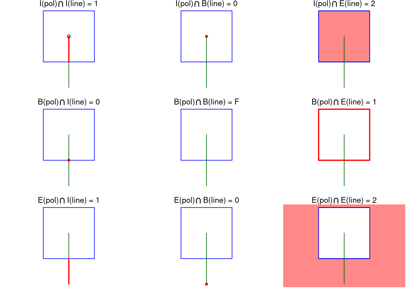
### Binary predicates and DE-9IM {#sec-de9im}
\index{geometry!predicates!binary}
\index{geometry!DE-9IM}
\index{DE-9IM}
The Dimensionally Extended Nine-Intersection Model [DE-9IM,
@de9im1; @de9im2] is a model that describes the qualitative
relation between any two geometries in two-dimensional space
($R^2$). Any geometry has a _dimension_ value that is:
* 0 for points,
* 1 for linear geometries,
* 2 for polygonal geometries, and
* F (false) for empty geometries
Any geometry also has an inside (I), a boundary (B), and an exterior (E); these
roles are obvious for polygons, however, for:
* **lines** the boundary is formed by the end points, and the inside
by all non-end points on the line
* **points** have a zero-dimensional inside but no boundary
```{r fig-de9im, fig.cap = "DE-9IM: intersections between the interior, boundary, and exterior of a polygon (rows) and of a linestring (columns) indicated by red", echo=!knitr::is_latex_output() }
#| code-fold: true
library(sf)
polygon <- po <- st_polygon(list(rbind(c(0,0), c(1,0), c(1,1), c(0,1), c(0,0))))
p0 <- st_polygon(list(rbind(c(-1,-1), c(2,-1), c(2,2), c(-1,2), c(-1,-1))))
line <- li <- st_linestring(rbind(c(.5, -.5), c(.5, 0.5)))
s <- st_sfc(po, li)

par(mfrow = c(3,3))
par(mar = c(1,1,1,1))

# "1020F1102"
# 1: 1
plot(s, col = c(NA, 'darkgreen'), border = 'blue', main = expression(paste("I(pol)",intersect(),"I(line) = 1")))
lines(rbind(c(.5,0), c(.5,.495)), col = 'red', lwd = 2)
points(0.5, 0.5, pch = 1)

# 2: 0
plot(s, col = c(NA, 'darkgreen'), border = 'blue', main = expression(paste("I(pol)",intersect(),"B(line) = 0")))
points(0.5, 0.5, col = 'red', pch = 16)

# 3: 2
plot(s, col = c(NA, 'darkgreen'), border = 'blue', main = expression(paste("I(pol)",intersect(),"E(line) = 2")))
plot(po, col = '#ff8888', add = TRUE)
plot(s, col = c(NA, 'darkgreen'), border = 'blue', add = TRUE)

# 4: 0
plot(s, col = c(NA, 'darkgreen'), border = 'blue', main = expression(paste("B(pol)",intersect(),"I(line) = 0")))
points(.5, 0, col = 'red', pch = 16)

# 5: F
plot(s, col = c(NA, 'darkgreen'), border = 'blue', main = expression(paste("B(pol)",intersect(),"B(line) = F")))

# 6: 1
plot(s, col = c(NA, 'darkgreen'), border = 'blue', main = expression(paste("B(pol)",intersect(),"E(line) = 1")))
plot(po, border = 'red', col = NA, add = TRUE, lwd = 2)

# 7: 1
plot(s, col = c(NA, 'darkgreen'), border = 'blue', main = expression(paste("E(pol)",intersect(),"I(line) = 1")))
lines(rbind(c(.5, -.5), c(.5, 0)), col = 'red', lwd = 2)

# 8: 0
plot(s, col = c(NA, 'darkgreen'), border = 'blue', main = expression(paste("E(pol)",intersect(),"B(line) = 0")))
points(.5, -.5, col = 'red', pch = 16)

# 9: 2
plot(s, col = c(NA, 'darkgreen'), border = 'blue', main = expression(paste("E(pol)",intersect(),"E(line) = 2")))
plot(p0 / po, col = '#ff8888', add = TRUE)
plot(s, col = c(NA, 'darkgreen'), border = 'blue', add = TRUE)
```
@fig-de9im shows the intersections between the I,
B, and E components of a polygon and a linestring indicated by red;
the sub-plot title gives the dimension of these intersections (0,
1, 2 or F). The relationship between the polygon and the line geometry is the
concatenation of these dimensions:
::: panel-tabset
#### R
```{r echo=!knitr::is_latex_output()}
#| code-fold: true
#| collapse: false
st_relate(polygon, line)
```
#### Python
```{python}
#| code-fold: true
#| collapse: false
from shapely.geometry import Polygon, LineString

polygon = Polygon([(0,0), (1,0), (1,1), (0,1), (0,0)])
line = LineString([(0.5, -0.5), (0.5, 0.5)])

# Find the spatial relationship between the polygon and line string
relation = polygon.relate(line)
print(relation)
```
:::
where the first three characters are associated with the inside
of the _first_ geometry (polygon): @fig-de9im is
summarised row-wise.
Using this ability to express relationships, we can also query
pairs of geometries about particular conditions expressed in a
_mask string_. As an example, the string `"*0*******"` would evaluate `TRUE`
when the second geometry has one or more boundary _points_ in common
with the interior of the first geometry; the symbol `*` standing for
"any dimensionality" (0, 1, 2 or F). The mask string `"T********"`
matches pairs of geometry with intersecting interiors, where the
symbol `T` stands for any non-empty intersection of dimensionality 0,
1, or 2.
Binary predicates are further described using normal-language verbs,
using DE-9IM definitions. For instance, the predicate `equals`
corresponds to the relationship `"T*F**FFF*"`. If any two geometries
obey this relationship, they are (topologically) equal, but may
have a different ordering of nodes.
A list of binary predicates, with their meaning for non-empty geometries:
|predicate |meaning of A _predicate_ B |inverse of |
|------------------------------|-----------------------------------------------------------------|----------------|
|`contains` |B has no points in the exterior of A _and_ the insides of A and B have at least one point in common| `within`|
|`contains_properly` |A contains B _and_ B has no points in common with the boundary of A| |
|`covers` |B has no points in the exterior of A| `covered_by`|
|`covered_by` |Inverse of `covers`| `covers`|
|`crosses` |A and B have some but not all interior points in common| |
|`disjoint` |A and B have no points in common| `intersects`|
|`equals` |A and B are topologically equal: node order or number of nodes may differ; identical to A contains B _and_ A within B|
|`equals_exact` |A equal B _and_ A and B have identical node order| |
|`intersects` |A and B are not disjoint| `disjoint`|
|`is_within_distance` |the shortest distance from A to B is within a given distance|
|`within` |A has no points in the exterior of B, _and_ the insides of A and B have at least one point in common| `contains`|
|`touches` |A and B have at least one boundary point but no interior points in common| |
|`overlaps` |A and B have the same dimension and some but not all points in common; the dimension of the common points is identical to that of A and B| |
|`relate` |Given a mask string, return whether A _relate_ B adheres to its pattern| |
\index[function]{st\_contains}
\index[function]{st\_contains\_properly}
\index[function]{st\_covers}
\index[function]{st\_covered\_by}
\index[function]{st\_crosses}
\index[function]{st\_disjoint}
\index[function]{st\_equals}
\index[function]{st\_equals\_exact}
\index[function]{st\_intersects}
\index[function]{st\_is\_within\_distance}
\index[function]{st\_within}
\index[function]{st\_touches}
\index[function]{st\_overlaps}
\index[function]{st\_relate}
The [Wikipedia DE-9IM page](https://en.wikipedia.org/wiki/DE-9IM)
provides the `relate` patterns for each of these verbs. They are
important to check out; for instance _covers_ and _contains_ (and
their inverses) are often not completely intuitive:
* if A _contains_ B, B has no points in common with the exterior _or
boundary_ of A
* if A _covers_ B, B has no points in common with the exterior of A
This implies for instance that a polygon covers its own boundary, but
does not contain it.
### Unary measures
\index{geometry!measures!unary}
Unary measures return a measure or quantity that describes a property of
the geometry:
|measure |returns |
|---------------------|--------------------------------------------------------------|
|`dimension` |0 for points, 1 for linear, 2 for polygons, possibly `NA` for empty geometries|
|`area` |the area of a geometry|
|`length` |the length of a linear geometry|
\index[function]{st\_dimension}
\index[function]{st\_area}
\index[function]{st\_length}
### Binary measures
\index{geometry!measures!binary}
`distance` returns the distance between pairs of geometries.
The qualitative measure `relate` (without mask) gives the relation
pattern. A description of the geometrical relationship between two
geometries is given in @sec-de9im.
\index[function]{st\_distance}
\index[function]{st\_relate}
### Unary transformers
\index{geometry!transformers!unary}
Unary transformations work on a per-geometry basis, and return for each geometry a new geometry.
|transformer |returns a geometry ... |
|-----------------------------|----------------------------------------------------------------------------------|
|`centroid`|of type `POINT` with the geometry's centroid|
|`buffer`|that is larger (or smaller) than the input geometry, depending on the buffer size|
|`jitter` |that was moved in space a certain amount, using a bivariate uniform distribution|
|`wrap_dateline`|cut into pieces that no longer cover or cross the dateline|
|`boundary`|with the boundary of the input geometry|
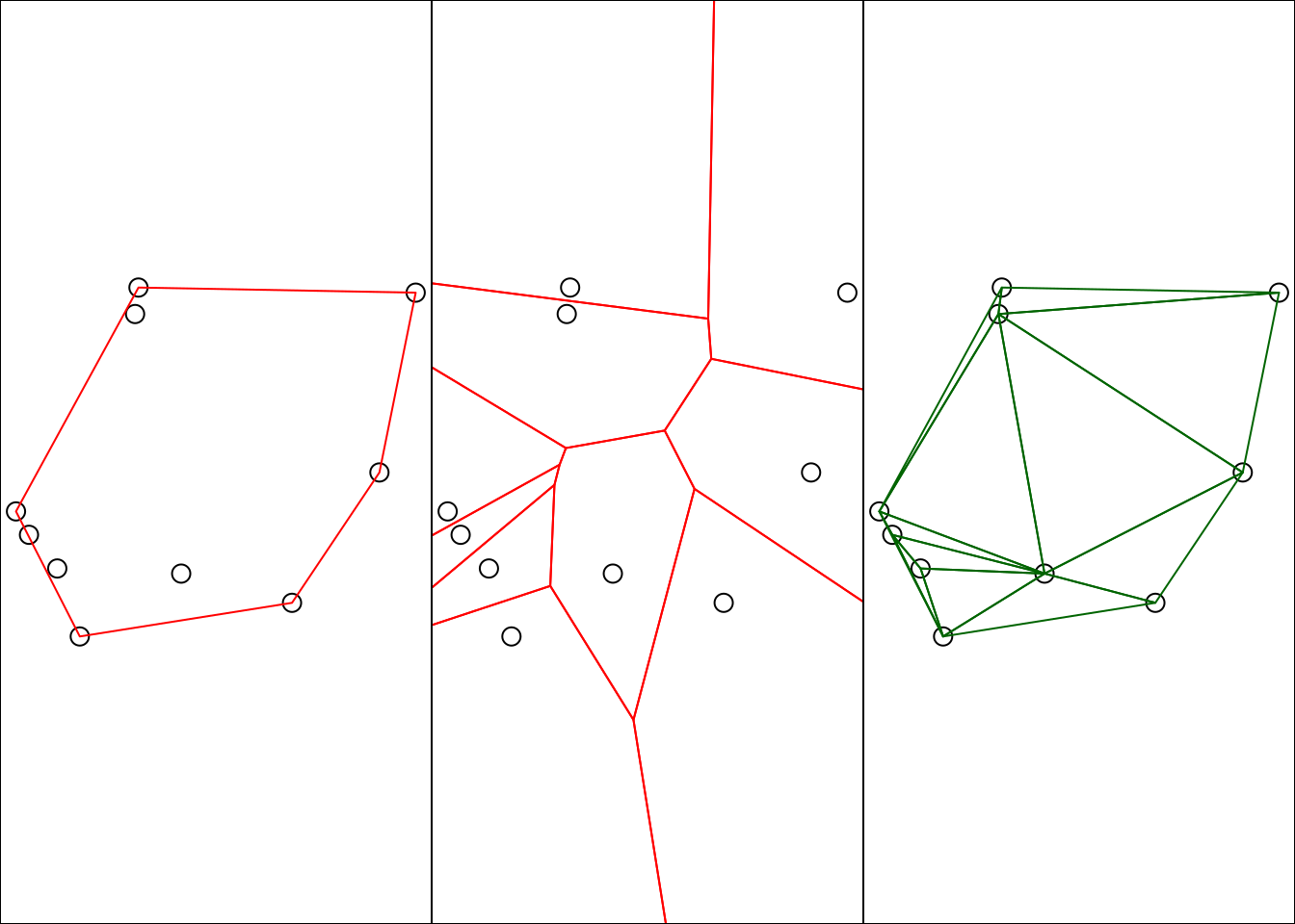
|`convex_hull`|that forms the convex hull of the input geometry (@fig-vor) |
|`line_merge`|after merging connecting `LINESTRING` elements of a `MULTILINESTRING` into longer `LINESTRING`s.|
|`make_valid`|that is valid |
|`node`|with added nodes to linear geometries at intersections without a node; only works on individual linear geometries|
|`point_on_surface`|with a (arbitrary) point on a surface|
|`polygonize`|of type polygon, created from lines that form a closed ring|
|`segmentize`|a (linear) geometry with nodes at a given density or minimal distance|
|`simplify`|simplified by removing vertices/nodes (lines or polygons)|
|`split`|that has been split with a splitting linestring|
|`transform`|transformed or convert to a new coordinate reference system (@sec-cs)|
|`triangulate`|with Delauney triangulated polygon(s) (@fig-vor) |
|`voronoi`|with the Voronoi tessellation of an input geometry (@fig-vor) |
|`zm`|with removed or added `Z` and/or `M` coordinates|
|`collection_extract`|with sub-geometries from a `GEOMETRYCOLLECTION` of a particular type|
|`cast`|that is converted to another type|
|`+`|that is shifted over a given vector|
|`*`|that is multiplied by a scalar or matrix|
```{r fig-vor, echo = !knitr::is_latex_output()}
#| fig.cap: "For a set of points, left: convex hull (red); middle: Voronoi polygons; right: Delauney triangulation"
#| code-fold: true
#| out.width: 60%
par(mar = rep(0,4), mfrow = c(1, 3))
set.seed(133331)
mp <- st_multipoint(matrix(runif(20), 10))
plot(mp, cex = 2)
plot(st_convex_hull(mp), add = TRUE, col = NA, border = 'red')
box()
plot(mp, cex = 2)
plot(st_voronoi(mp), add = TRUE, col = NA, border = 'red')
box()
plot(mp, cex = 2)
plot(st_triangulate(mp), add = TRUE, col = NA, border = 'darkgreen')
box()
```
\index[function]{st\_centroid}
\index[function]{st\_buffer}
\index[function]{st\_jitter}
\index[function]{st\_wrap\_dateline}
\index[function]{st\_boundary}
\index[function]{st\_convex\_hull}
\index[function]{st\_line\_merge}
\index[function]{st\_make\_valid}
\index[function]{st\_node}
\index[function]{st\_point\_on\_surface}
\index[function]{st\_polygonize}
\index[function]{st\_segmentize}
\index[function]{st\_simplify}
\index[function]{st\_split}
\index[function]{st\_transform}
\index[function]{st\_triangulate}
\index[function]{st\_voronoi}
\index[function]{st\_zm}
\index[function]{st\_collection\_extract}
\index[function]{st\_cast}
### Binary transformers {#sec-bintrans}
\index{geometry!transformers!binary}
Binary transformers are functions that return a geometry based on
operating on a pair of geometries. They include:
|function |returns |infix operator|
|-------------------|-----------------------------------------------------------|:------------:|
|`intersection` |the overlapping geometries for pair of geometries |`&`|
|`union` |the combination of the geometries; removes internal boundaries and duplicate points, nodes or line pieces|`|`|
|`difference` |the geometries of the first after removing the overlap with the second geometry|`/`|
|`sym_difference` |the combinations of the geometries after removing where they intersect; the negation (opposite) of `intersection`|`%/%`|
\index[function]{st\_intersection}
\index[function]{st\_union}
\index[function]{st\_difference}
\index[function]{st\_sym\_difference}
### N-ary transformers {#sec-nary}
\index{geometry!transformers!n-ary}
N-ary transformers operate on sets of geometries.
`union` can be applied to a set of geometries to return its
geometrical union. Otherwise, any set of geometries can be combined
into a `MULTI`-type geometry when they have equal dimension, or
else into a `GEOMETRYCOLLECTION`. Without unioning, this may
lead to a geometry that is not valid, for instance when two polygon
rings have a boundary line in common.
\index[function]{st\_union!n-ary}
\index[function]{st\_intersection!n-ary}
\index[function]{st\_difference!n-ary}
N-ary `intersection` and `difference` take a single argument
but operate (sequentially) on all pairs, triples, quadruples, etc.
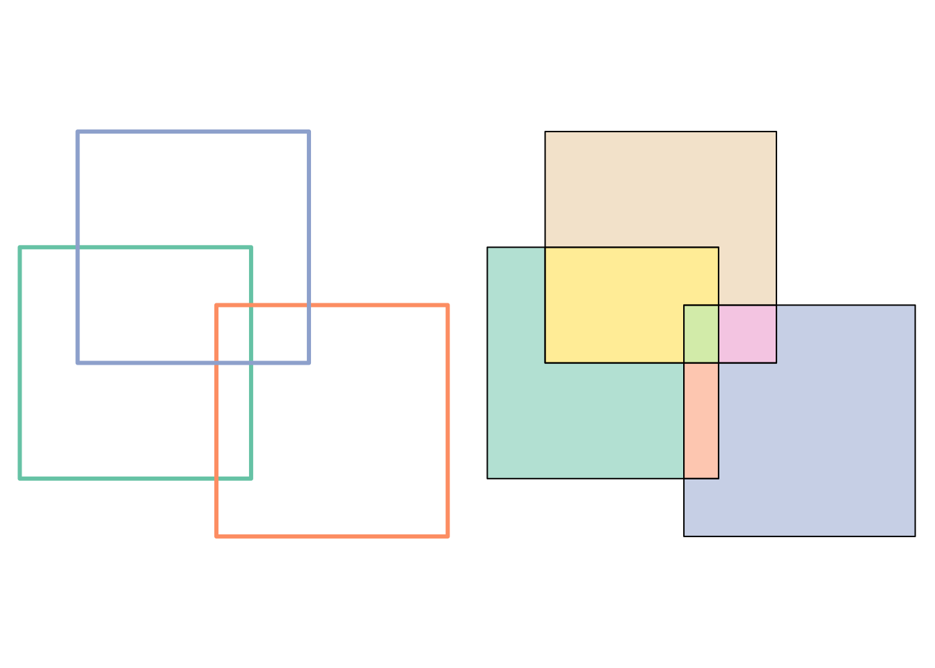
Consider the plot in @fig-boxes: how do we identify
the area where all three boxes overlap? Using binary intersections
gives us intersections for all pairs: 1-1, 1-2, 1-3, 2-1, 2-2, 2-3,
3-1, 3-2, 3-3, but that does not let us identify areas where more than
two geometries intersect.
@fig-boxes (right) shows the n-ary intersection: the seven
unique, non-overlapping geometries originating from intersection
of one, two, _or more_ geometries.
```{r fig-boxes, eval=TRUE, echo=!knitr::is_latex_output()}
#| code-fold: true
#| out.width: 50%
#| fig.cap: "Left: three overlapping squares -- how do we identify the small box where all three overlap? Right: unique, non-overlapping n-ary intersections"
par(mar = rep(.1, 4), mfrow = c(1, 2))
sq <- function(pt, sz = 1) st_polygon(list(rbind(c(pt - sz),
  c(pt[1] + sz, pt[2] - sz), c(pt + sz), c(pt[1] - sz, pt[2] + sz), c(pt - sz))))
x <- st_sf(box = 1:3, st_sfc(sq(c(0, 0)), sq(c(1.7, -0.5)), sq(c(0.5, 1))))
plot(st_geometry(x), col = NA, border = sf.colors(3, categorical = TRUE), lwd = 3)
plot(st_intersection(st_geometry(x)), col = sf.colors(7, categorical=TRUE, alpha = .5))
```
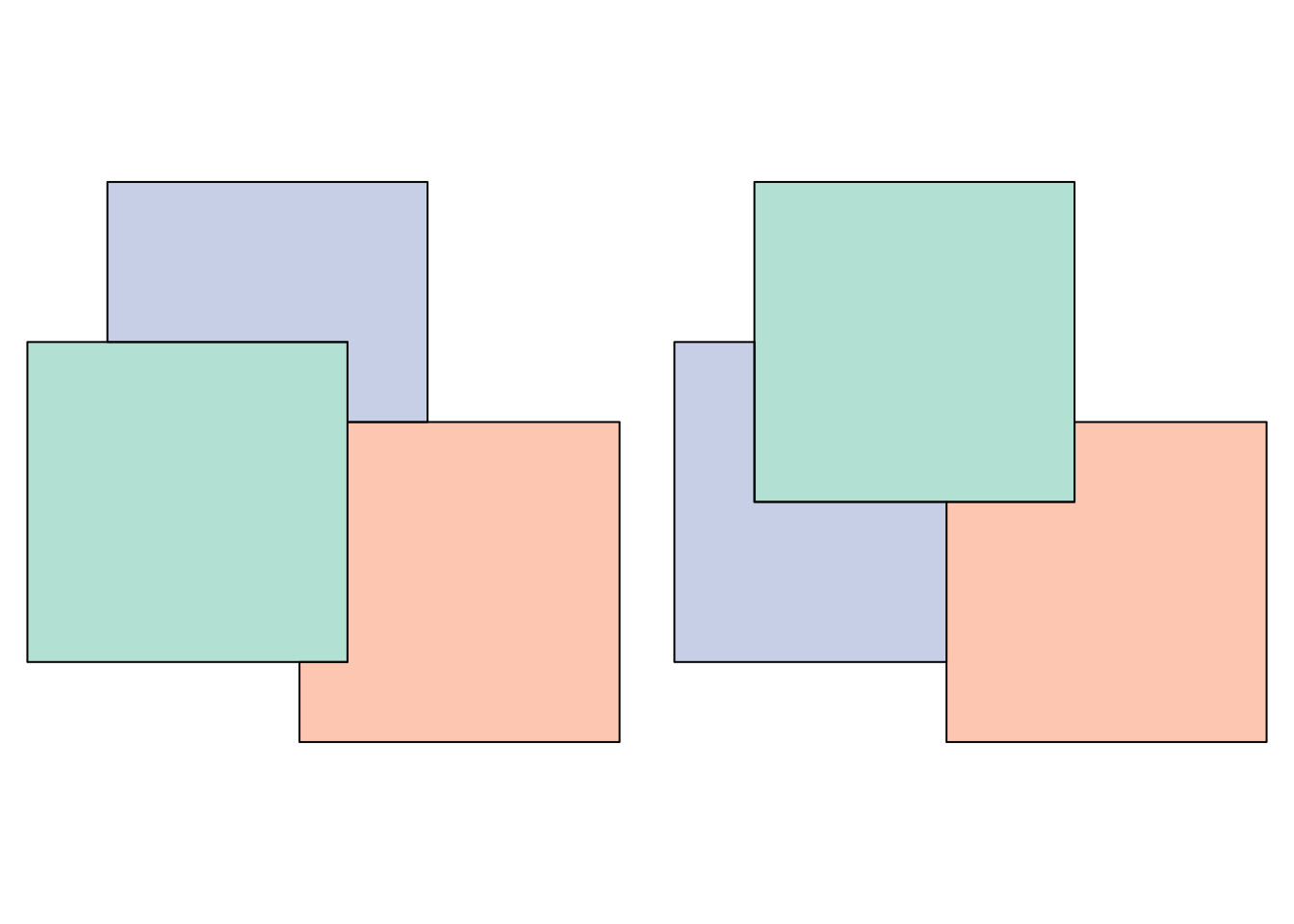
Similarly, one can compute an n-ary _difference_ from a set $\{s_1, s_2,
s_3, ...\}$ by creating differences $\{s_1, s_2-s_1, s_3-s_2-s_1,
...\}$. This is shown in @fig-diff, (left) for the original
set, and (right) for the set after reversing its order to make clear that
the result here depends on the ordering of the input geometries. Again,
resulting geometries do not overlap.
```{r fig-diff, echo=!knitr::is_latex_output()}
#| code-fold: true
#| out.width: 50%
#| fig.cap: "Difference between subsequent boxes, left: in original order; right: in reverse order"
par(mar = rep(.1, 4), mfrow = c(1, 2))
xg <- st_geometry(x)
plot(st_difference(xg), col = sf.colors(3, alpha = .5, categorical=TRUE))
plot(st_difference(xg[3:1]), col = sf.colors(3, alpha = .5, categorical=TRUE))
```
## Precision {#sec-precision}
\index{precisions}
\index{coordinates!precisions}
\index[function]{st\_precision}
Geometrical operations, such as finding out whether a certain
point is on a line, may fail when coordinates are represented by
double precision floating point numbers, such as 8-byte doubles
used in R. An often chosen remedy is to limit the precision of the
coordinates before the operation. For this, a _precision model_
is adopted; the most common is to choose a factor $p$ and compute
rounded coordinates $c'$ from original coordinates $c$ by
$$c' = \mbox{round}(p \cdot c) / p$$
Rounding of this kind brings the coordinates to points on a
regular grid with spacing $1/p$, which is beneficial for geometric
computations. Of course, it also affects all computations like
areas and distances, and may turn valid geometries into invalid
ones. Which precision values are best for which application is
often a matter of common sense combined with trial and error.
## Coverages: tessellations and rasters {#sec-coverages}
\index{coverage}
The Open Geospatial Consortium defines a _coverage_ as a "feature
that acts as a function to return values from its range for any
direct position within its spatiotemporal domain" [@ogccov]. Having
a _function_ implies that for every space time "point", every combination
of a spatial point and a moment in time of the spatiotemporal domain,
we have a _single_ value for the range. This is a very common situation
for spatiotemporal phenomena, a few examples can be given:
* boundary disputes aside, at a given time every point in a region (domain) belongs to a single administrative unit (range)
* at any given moment in time, every point in a region (domain) has a certain _land cover type_ (range)
* every point in an area (domain) has a single surface elevation (range), which could be measured with respect to a given mean sea level surface
* every spatiotemporal point in a three-dimensional body of air (domain) has single value for temperature (range)
A caveat here is that because observation or measurement always takes
time and requires space, measured values are always an average over
a spatiotemporal volume, and hence range variables can rarely be
measured for true, zero-volume "points"; for many practical cases
however the measured volume is small enough to be considered a
"point". For a variable like _land cover type_ the volume needs to
be chosen such that the types distinguished make sense with respect
to the measured areal units.
In the first two of the given examples the range variable is
_categorical_, in the last two the range variable is _continuous_.
For categorical range variables, if large connected areas have a
constant range value, an efficient way to represent these data
is by storing the boundaries of the areas with constant value, such
as country boundaries. Although this can be done (and is often done)
by a set of simple feature geometries (polygons or multi-polygons),
this brings along some challenges:
* it is hard to guarantee for such a set of simple feature polygons that they do not overlap, or that there are no unwanted gaps between them
* simple features have no way of assigning points _on_ the boundary of two adjacent polygons uniquely to a single polygon, which conflicts with the interpretation as coverage
### Topological models
\index{topology}
A data model that guarantees no inadvertent gaps or overlaps of
polygonal coverages is the _topological_ model, examples of which
are found in geographic information systems (GIS) like GRASS GIS
or ArcGIS. Topological models store boundaries between polygons
only once and register which polygonal area is on either side
of a boundary.
Deriving the set of (multi)polygons for each area with a constant
range value from a topological model is straightforward; the other
way around, reconstructing topology from a set of polygons typically
involves setting thresholds on errors and handling gaps or overlaps.
### Raster tessellations
\index{tesselation}
\index{coverage!tesselation}
\index{polygon!tesselation}
\index{raster!tesselation}
A tessellation is a sub-division of a space (area, volume) into
smaller elements by ways of polygons. A regular tessellation
does this with regular polygons: triangles, squares, or hexagons.
Tessellations using squares are commonly used for spatial data
and are called _raster data_. Raster data
tessellate each spatial dimension $d$ into regular cells,
formed by left-closed and right-open intervals $d_i$:
\begin{equation}
d_i = d_0 + [i \times \delta, (i+1) \times \delta)
\end{equation}
with $d_0$ an offset, $\delta$ the interval (cell or
pixel) size, and where the cell index $i$ is an arbitrary but
consecutive set of integers. The $\delta$ value is often taken
negative for the $y$-axis (Northing), indicating that raster
row numbers increasing Southwards correspond to $y$-coordinates
increasing Northwards.
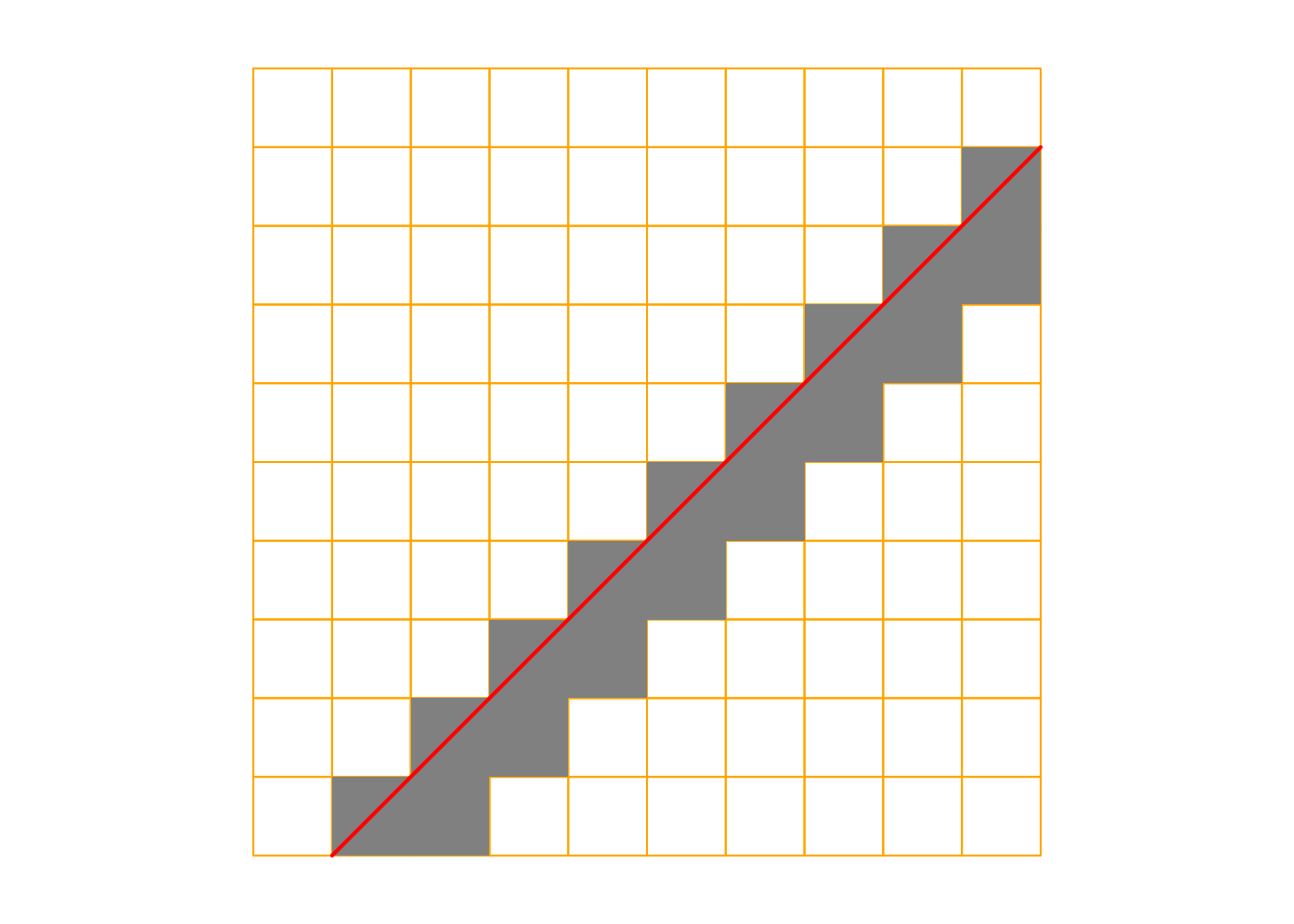
Whereas in arbitrary polygon tessellations the assignment of points
to polygons is ambiguous for points falling on a boundary shared
by two polygons, using left-closed "[" and right-open ")" intervals
in regular tessellations removes this ambiguity. This means that for
rasters with negative $\delta$ values for the $y$-coordinate and
positive for the $x$-coordinate, only the top-left corner point
is part of each raster cell. An artifact resulting from this is
shown in @fig-rasterizeline.
```{r fig-rasterizeline, echo=!knitr::is_latex_output()}
#| out.width: 50%
#| fig.cap: "Rasterization artifact: as only top-left corners are part of the raster cell, only cells touching the red line below the diagonal line are rasterized"
#| code-fold: true
library(stars) |> suppressPackageStartupMessages()
par(mar = rep(1, 4))
ls <- st_sf(a = 2, st_sfc(st_linestring(rbind(c(0.1, 0), c(1, .9)))))
grd <- st_as_stars(st_bbox(ls), nx = 10, ny = 10, xlim = c(0, 1.0), ylim = c(0, 1),
   values = -1)
r <- st_rasterize(ls, grd, options = "ALL_TOUCHED=TRUE")
r[r == -1] <- NA
plot(st_geometry(st_as_sf(grd)), border = 'orange', col = NA,
     reset = FALSE, key.pos = NULL)
plot(r, axes = FALSE, add = TRUE, breaks = "equal", main = NA) # ALL_TOUCHED=FALSE;
plot(ls, add = TRUE, col = "red", lwd = 2)
```
\index{tesselation!time}
Tessellating the time dimension with left-closed right-open intervals
is very common, and it reflects the implicit assumption underlying
time series software such as the **xts** package in R, where time
stamps indicate the start of time intervals. Different models can
be combined: one could use simple feature polygons to tessellate
space and combine this with a regular tessellation of time in order
to cover a space time _vector data cube_. Raster and vector data
cubes are discussed in @sec-datacube.
As mentioned above, besides square cells the other two shapes
that can lead to regular tessellations of $R^2$ are triangles
and hexagons. On the sphere, there are a few more, including cube,
octahedron, icosahedron, and dodecahedron. A spatial index that
builds on the cube is [s2geometry](https://s2geometry.io/), the
[H3 library](https://eng.uber.com/h3/) uses the icosahedron and
densifies that with (mostly) hexagons. Mosaics that cover the entire
Earth are also called _discrete global grids_.
## Networks
\index{networks}
Spatial networks [@barthelemy2011spatial] are typically composed of linear (`LINESTRING`)
elements, but possess further topological properties describing
the network coherence:
* start- and end-points of a linestring may be connected to other linestring
start or end points, forming a set of nodes and edges
* edges may be directed, to only allow for connection (flow,
transport) in one way
R packages including **osmar** [@R-osmar], **stplanr** [@R-stplanr], and
**sfnetworks** [@R-sfnetworks] provide functionality for constructing
network objects, and working with them, including computation of shortest or
fastest routes through a network. Package **spatstat** [@R-spatstat;
@baddeley2015spatial] has infrastructure for analysing point
patterns on linear networks (@sec-pointpatterns). Chapter 12 of
@geocomp has a transportation application using networks.
## Exercises
For the following exercises, use R where possible.
1. Give two examples of geometries in 2-D (flat) space that cannot be represented as simple feature geometries, and create a plot of them.
2. Recompute the coordinates 10.542, 0.01, 45321.6789 using precision values 1, 1e3, 1e6, and 1e-2.
3. Describe a practical problem for which an n-ary intersection would be needed.
4. How can you create a Voronoi diagram (@fig-vor) that has one closed polygons for every single point?
5. Give the unary measure `dimension` for geometries `POINT Z (0 1 1)`, `LINESTRING Z (0 0 1,1 1 2)`, and `POLYGON Z ((0 0 0,1 0 0,1 1 0,0 0 0))`
6. Give the DE-9IM relation between `LINESTRING(0 0,1 0)` and `LINESTRING(0.5 0,0.5 1)`; explain the individual characters.
7. Can a set of simple feature polygons form a coverage? If so, under which constraints?
8. For the `nc` counties in the dataset that comes with R package **sf**, find the points touched by four counties.
9. How would @fig-rasterizeline look like if $\delta$ for the $y$-coordinate was positive?