# Attributes and Support {#sec-featureattributes}
\index{support}
\index{geometry!support}
Feature _attributes_ refer to the properties of features ("things")
that do not describe the feature's geometry. Feature attributes can
be _derived_ from geometry (such as length of a `LINESTRING` or area
of a `POLYGON`), but they can also refer to non-derived properties,
such as:
* name of a street or county
* number of people living in a country
* type of a road
* soil type in a polygon from a soil map
* opening hours of a shop
* body weight or heart beat rate of an animal
* NO$_2$ concentration measured at an air quality monitoring station
In some cases, time properties can be seen as attributes of
features, for instance the date of birth of a person or the construction
year of a road. When an attribute such as for instance air quality
is a function of both space and time, time is best handled on
equal footing with geometry (often in a data cube, see
@sec-datacube).
Spatial data science software implementing simple features
typically organises data in tables that contain both geometries and
attributes for features; this is true for `geopandas` in Python,
`PostGIS` tables in PostgreSQL, and `sf` objects in R. The geometric
operations described in @sec-opgeom operate
on geometries _only_, and may occasionally yield new attributes
(predicates, measures, or transformations), but they do not operate
on attributes present.
When, while manipulating geometries, attribute _values_ are retained
unmodified, support problems may arise.
If we look into a simple case of replacing a county polygon with
the centroid of that polygon on a dataset that has attributes,
we see that R package **sf** issues a warning:
```{r fig-countycentroid, cache = FALSE, echo = !knitr::is_latex_output()}
#| code-fold: true
#| collapse: false
library(sf) |> suppressPackageStartupMessages()
library(dplyr) |> suppressPackageStartupMessages()
system.file("gpkg/nc.gpkg", package="sf") |>
    read_sf() |>
    st_transform(32119) |>
    select(BIR74, SID74, NAME) |>
    st_centroid() -> x
```
\newpage
The reason for this is that the dataset contains variables with
values that are associated with entire polygons -- in this case
population counts -- meaning they are not associated with a
`POINT` geometry replacing the polygon.
\index{warning!assumes attributes are constant over geometries of x}
In @sec-support we already described that for non-point
geometries (lines, polygons), feature attribute values either
have _point support_, meaning that the value applies to _every
point_, or they have _block support_, meaning that the value
_summarises all points_ in the geometry. (Other options,
non-point support smaller than the geometry, or support larger
than the associated geometry, may also occur.) This chapter
will describe different ways in which an attribute may relate to
the geometry, its consequences on analysing such data, and ways to
derive attribute data for different geometries (up- and downscaling).
\index{support!point}
\index{support!block}
\index{support!upscaling}
\index{support!downscaling}
## Attribute-geometry relationships and support {#sec-agr}
\index{attribute-geometry relationship}
\index{geometry!relationship to attribute}
\index[function]{st\_agr}
Changing the feature geometry without changing the feature attributes
does change the _feature_, since the feature is characterised by
the combination of geometry and attributes. Can we, ahead of time,
predict whether the resulting feature will still meaningfully relate
to the attribute value when we replace all geometries for instance
with their convex hull or centroid? It depends.
Take the example of a road, represented by a `LINESTRING`, which has
an attribute property _road width_ equal to 10 m. What can we say about
the road width of an arbitrary sub-section of this road? That depends
on whether the attribute road length describes, for instance the
road width _everywhere_, meaning that road width is constant along the
road, or whether it describes an aggregate property, such as minimum
or average road width. In case of the minimum, for an arbitrary
subsection of the road one could still argue that the minimum
road width must be at least as large as the minimum road width for
the whole segment, but it may no longer be _the minimum_ for that
subsection. This gives us two "types" for the attribute-geometry
relationship (**AGR**):
* **constant** the attribute value is valid everywhere in or over the
geometry; we can think of the feature as consisting of an infinite
number of points that all have this attribute value; in geostatistical
terminology this is known as a variable with _point support_
* **aggregate** the attribute is an aggregate, a summary value over
the geometry; we can think of the feature as a _single_ observation
with a value that is associated with the _entire_ geometry; this is
also known as a variable having _block support_
\index{attribute-geometry relationship!constant}
\index{attribute-geometry relationship!aggregate}
For polygon data, typical examples of **constant** AGR (point
support) variables are:
* land use for a land use polygon
* rock units or geologic strata in a geological map
* soil type in a soil map
* elevation class in an elevation map that shows elevation as classes
* climate zone in a climate zone map
A typical property of such variables is that they have geometries
that are not man-made and also not associated with a sensor device
(such as remote sensing image pixel boundaries). Instead, the geometry
follows from mapping the variable observed.
Examples for the **aggregate** AGR (block support) variables are:
* population, either as number of persons or as population density
* other socio-economic variables, summarised by area
* average reflectance over a remote sensing pixel
* total emission of pollutants by region
* block mean NO$_2$ concentrations, such as obtained by block kriging
over square blocks (@sec-blockkriging) or by a dispersion model that
predicts areal means
A typical property of such variables is that associated geometries
come for instance from legislation, observation devices or analysis
choices, but not intrinsically from the observed variable.
\index{attribute-geometry relationship!identity}
A third type of AGR arises when an attribute _identifies_ a feature
geometry; we call an attribute an **identity** variable when
the associated geometry uniquely identifies the variable's value
(there are no other geometries with the same value). An example is
county name: the name identifies the county, and is still the county
for any sub-area (point support), but for arbitrary sub-areas, the
attributes loses the **identity** property to become a **constant**
attribute. An example is:
* an arbitrary point (or region) inside a county is still part of the
county and must have the same value for county name, but it no
longer identifies the (entire) geometry corresponding to that county
The challenge here is that spatial information (ignoring time for
simplicity) belongs to different phenomena types [@scheider2016],
including:
* **fields**: where over _continuous_ space, every location corresponds to a single value, examples including elevation, air quality, or land use
* **objects**: found at a _discrete_ set of locations, such as houses, trees, or persons
* **aggregates**: values arising as spatial sums, totals, or averages of fields, counts or densities of objects, associated with lines or regions
\index{fields}
\index{objects}
\index{aggregates}
but that different spatial geometry types (points, lines, polygons,
raster cells) have no simple mapping to these phenomena types:
* points may refer to sample locations of observations on fields (air quality) or to locations of objects
* lines may be used for objects (roads, rivers), contours of a field, or administrative borders
* raster pixels and polygons may reflect fields of a categorical
variable such as land use (_coverage_), but also aggregates such
as population density
* raster or other mesh triangulations may have different variables
associated with nodes (points), edges (lines), or faces
(areas, cells), for instance when partial differential equations
are approximated using _staggered grids_ [@Haltiner; @Collins13]
Properly specifying attribute-geometry relationships, and warning
against their absence or cases when change in geometry (change
of support) implies a change of information can help to avoid a
large class of common spatial data analysis mistakes [@stasch2014]
associated with the _support_ of spatial data.
## Aggregating and summarising
Aggregating records in a table (or `data.frame`) involves two steps:
* grouping records based on a grouping predicate, and
* applying an aggregation function to the attribute values of a
group to summarise them into a single number.
In SQL, this looks for instance like
```
SELECT GroupID, SUM(population) FROM table GROUP BY GroupID;
```
indicating the aggregation _function_ (`SUM`) and the
_grouping predicate_ (`GroupID`).
R package **dplyr** for instance uses two steps to accomplish this:
function `group_by` specifies the group membership of records,
`summarise` computes data summaries (such as `sum` or `mean`)
for each of the groups. The (base) R method `aggregate` combines
both in a single function call that takes the table, the grouping
predicate(s), and the aggregation function(s) as arguments.
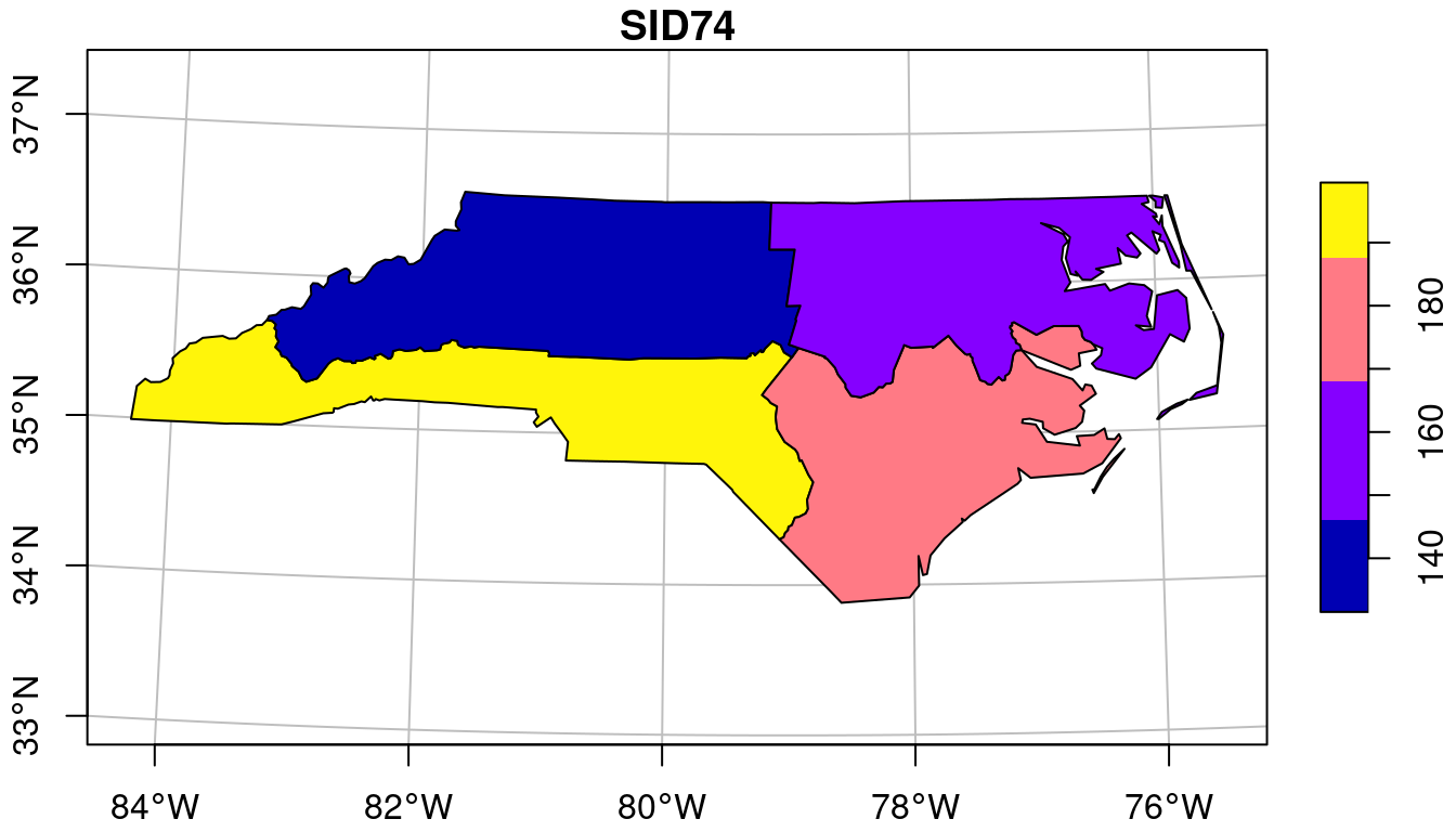
An example for the North Carolina counties is shown in
@fig-ncaggregation. Here, we grouped counties by their position
(according to the quadrant in which the county centroid is with
respect to ellipsoidal coordinate `POINT(-79, 35.5)`) and summed
the number of disease cases per group. The result shows that
the geometries of the resulting groups have been unioned
(@sec-bintrans): this is necessary because the `MULTIPOLYGON`
formed by just putting all the county geometries together would
have many duplicate boundaries, and hence would not be _valid_
(@sec-valid).
```{r fig-ncaggregation, echo = !knitr::is_latex_output()}
#| code-fold: true
#| fig.cap: "SID74 total incidences aggregated to four areas"
#| fig.height: 4
nc <- read_sf(system.file("gpkg/nc.gpkg", package = "sf"))
# encode quadrant by two logicals:
nc$lng <- st_coordinates(st_centroid(st_geometry(nc)))[,1] > -79
nc$lat <- st_coordinates(st_centroid(st_geometry(nc)))[,2] > 35.5
nc.grp <- aggregate(nc["SID74"], list(nc$lng, nc$lat), sum)
nc.grp["SID74"] |> st_transform('EPSG:32119') |>
  plot(graticule = TRUE, axes = TRUE)
```
Plotting collated county polygons is technically not a problem, but
for this case would raise the wrong suggestion that the group sums
relate to individual counties, rather than to the grouped counties.
One particular property of aggregation in this way is that each
record is assigned to a single group; this has the advantage that
the sum of the group-wise sums equals the sum of the un-grouped data:
for variables that reflect _amount_, nothing gets lost and nothing
is added. The newly formed geometry is the result of unioning the
geometries of the contributing records.
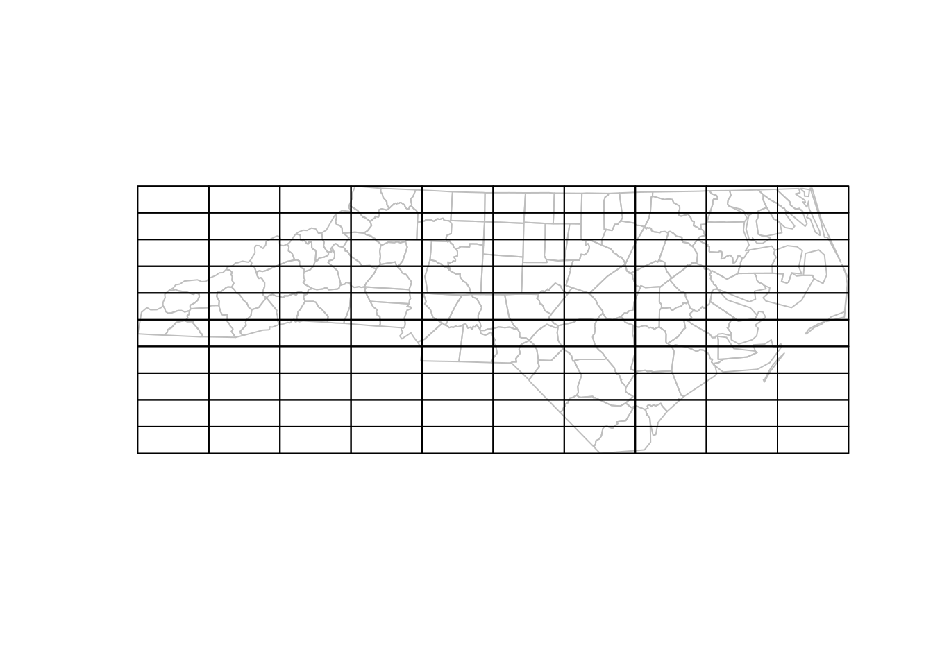
```{r fig-ncblocks, echo=!knitr::is_latex_output()}
#| fig.cap: "Example target blocks plotted over North Carolina counties"
#| code-fold: true
nc <- st_transform(nc, 2264)
gr <- st_sf(
   label = apply(expand.grid(1:10, LETTERS[10:1])[,2:1], 1, paste0, collapse = " "),
   geom = st_make_grid(nc))
plot(st_geometry(nc), reset = FALSE, border = 'grey')
plot(st_geometry(gr), add = TRUE)
```
When we need an aggregate for a new area that is _not_ a union of the
geometries for a group of records, and we use a spatial predicate,
then single records may be matched to multiple groups. When taking
the rectangles of @fig-ncblocks as the target areas,
and summing for each rectangle the disease cases of the counties
that _intersect_ with the rectangles of @fig-ncblocks,
the sum of these will be much larger:
```{r fig-aggnc, echo=!knitr::is_latex_output()}
#| code-fold: true
#| collapse: false
a <- aggregate(nc["SID74"], gr, sum)
c(sid74_sum_counties = sum(nc$SID74),
  sid74_sum_rectangles = sum(a$SID74, na.rm = TRUE))
```
Choosing another predicate, such as _contains_ or _covers_, would on
the contrary result in much smaller values, because many counties
are not contained by _any_ of the target geometries. However, there are
a few cases where this approach might be good or satisfactory:
* when we want to aggregate `POINT` geometries by a set of polygons,
and all points are contained by a single polygon. If points fall on a
shared boundary than they are assigned to both polygons (this is
the case for DE-9IM-based GEOS library; the s2geometry library has
the option to define polygons as "semi-open", which implies that
points are assigned to maximally one polygon when polygons do not
overlap)
* when aggregating many very small polygons or raster pixels over
larger areas, for instance _averaging_ altitude from a 30 m resolution raster
over North Carolina counties, the error made by multiple matches
may be insignificant
* when the many-to-many match is reduced to the single largest area
match, as shown in @fig-largest
A more comprehensive approach to aggregating spatial data associated
with areas to larger, arbitrary shaped areas is by using area-weighted
interpolation.
## Area-weighted interpolation and dasymetric mapping {#sec-area-weighted}
\index{area-weighted interpolation}
\index{interpolation!area-weighted}
\index{conservative region aggregation}
\index{conservative region regridding}
When we want to combine geometries and attributes of two datasets
such that we get attribute values of a source dataset summarised for
the geometries of a target, where source and target geometries are
unrelated, area-weighted interpolation may be a simple approach. In
effect, it considers the area of overlap of the source and target
geometries, and uses that to weigh the source attribute values into
the target value [@goodchild; @thomas; @do; @Do2021]. This method
is also known as conservative region aggregation or regridding
[@conservative]. Here, we follow the notation of @do.
Area-weighted interpolation computes, for each of $q$ spatial target
areas $T_j$, a weighted average from the values $Y_i$ corresponding
to the $p$ spatial source areas $S_i$,
$$
\hat{Y}_j(T_j) = \sum_{i=1}^p w_{ij} Y_i(S_i)
$$ {#eq-aw}
where the $w_{ij}$ depend on the amount of overlap of $T_j$ and
$S_i$, and the amount of overlap is $A_{ij} = T_j \cap S_i$. How
$w_{ij}$ depends on $A_{ij}$ is discussed below.
Different options exist for choosing weights, including methods
using external variables [including dasymetric mapping, @mennis].
Two simple approaches for computing weights that do not use external
variables arise, depending on whether the variable $Y$ is _intensive_
or _extensive_.
### Spatially extensive and intensive variables {#sec-extensiveintensive}
\index{extensive properties}
\index{intensive properties}
Extensive variables correspond to amounts, associated with a
physical size (length, area, volume, counts of items). An example
of a extensive variable is _population count_. It is associated with
an area, and if that area is cut into smaller areas, the population
count needs to be split too. Because population is rarely uniform
over space, this does not need to be done proportionally to the
smaller areas but the sum of the population count for the smaller
areas needs to equal that of the total. Intensive variables are
variables that do not have values proportional to support: if the
area is split, values may vary but _on average_ remain the same.
An example of a related variable that is _intensive_ is population
density. If an area is split into smaller areas, population density
is not split similarly: the _sum_ of population densities for the
smaller areas is a meaningless measure, as opposed to the _average_
of the population densities which will be similar to the density
of the total area.
When we assume that the **extensive** variable $Y$ is uniformly
distributed over space, the value $Y_{ij}$, derived from $Y_i$
for a sub-area of $S_i$, $A_{ij} = T_j \cap S_i$ of $S_i$ is
$$\hat{Y}_{ij}(A_{ij}) = \frac{|A_{ij}|}{|S_i|} Y_i(S_i)$$
where $|\cdot|$ denotes the spatial area.
For estimating $Y_j(T_j)$ we sum all the elements over area $T_j$:
$$
\hat{Y}_j(T_j) = \sum_{i=1}^p \frac{|A_{ij}|}{|S_i|} Y_i(S_i)
$$ {#eq-awextensive}
For an **intensive** variable, under the assumption that the variable
has a constant value over each area $S_i$, the estimate for a
sub-area equals that of the total area,
$$\hat{Y}_{ij} = Y_i(S_i)$$
and we can estimate the value of $Y$ for a new spatial unit $T_j$
by
$$
\hat{Y}_j(T_j) = \frac{1}{|T_j|} \sum_{i=1}^p |A_{ij}| Y_i(S_i)
$$ {#eq-awintensive}
which is an area-weighted average of the source values when
$\sum_{i=1}^p |A_{ij}|$ equals $|T_j|$. This is the case when
source regions completely cover all target regions. When (some
of) the target regions extend beyond the source regions there
are non-intersected areas, and dividing by $|T_j|$ could lead
to biased values. In that case, instead of dividing by $|T_j|$
in @eq-awintensive one would divide by $\sum_{i=1}^p |A_{ij}|$.
### Dasymetric mapping {#sec-dasymetric}
\index{dasymetric mapping}
Dasymetric mapping distributes variables known at a coarse spatial aggregation level,
such as population, over finer spatial
units by using another variable that is associated with population
distribution, such as land use, building density, or road density.
The simplest approach to dasymetric mapping is obtained for
extensive variables, where the area ratio $|A_{ij}| / |S_i|$ in
@eq-awextensive is replaced by the ratio of another extensive
variable $X_{ij}(S_{ij})/X_i(S_i)$, which has to be known for both
the intersecting regions $S_{ij}$ and the source regions $S_i$.
In case only $X_i(S_i)$ is available, e.g. on a fine regular grid, area-weighted
interpolation can be used to approximate the $X_{ij}(S_{ij})$.
@do discuss several alternatives for intensive $Y$ and/or $X$,
and cases where $X$ is known for other areas. Section @sec-sf-joins
provides a dasymetric mapping example.
### Support in file formats
\index{support!in file formats}
GDAL's vector API supports reading and writing so-called field
domains, which can have a "split policy" and a "merge policy"
indicating what should be done with attribute variables when
geometries are split or merged. The values of these can be
"duplicate" for split and "geometry weighted" for merge, in
case of spatially intensive variables, or they can be "geometry
ratio" for split and "sum" for merge, in case of spatially
extensive variables. At the time of writing this, the [file
formats supporting this](https://github.com/OSGeo/gdal/pull/3638)
are GeoPackage and FileGDB. @sdsl2026 contains a discussion about
the potential of ambiguous use of these field domain labels.
## Up- and Downscaling {#sec-updownscaling}
\index{upscaling}
\index{downscaling}
Up- and downscaling refers in general to obtaining high-resolution
information from low-resolution data (downscaling) or obtaining
low-resolution information from high-resolution data (upscaling).
Both activities involve the attributes' relation to geometries and
both change support. They are synonymous with aggregation (upscaling)
and disaggregation (downscaling). The simplest form of downscaling
is sampling (or extracting) polygon, line or grid cell values at
point locations. This works well for variables with point-support
("constant" AGR), but is at best approximate when the values are
aggregates. Challenging applications for downscaling include
high-resolution prediction of variables obtained by low-resolution
weather prediction models or climate change models, and the
high-resolution prediction of satellite image derived variables
based on the fusion of sensors with different spatial and temporal
resolutions.
The application of areal interpolation using (@eq-aw) with
its realisations for extensive (@eq-awextensive) and intensive
(@eq-awintensive) variables allows moving information from any
source area $S_i$ to any target area $T_j$ as long as the two areas
have some overlap. This means that one can go arbitrarily to much
larger units (aggregation) or to much smaller units (disaggregation).
Of course this makes only sense to the extent that the assumptions
hold: over the source regions extensive variables need to be
uniformly distributed and intensive variables need to have a
constant value.
The ultimate disaggregation involves retrieving (extracting)
point values from line or area data. For this, we cannot work with
equations -@eq-awextensive or -@eq-awintensive because
$|A_{ij}| = 0$ for points, but under the assumption of having a
constant value over the geometry, for intensive variables the value
$Y_i(S_i)$ can be assigned to points as long as all points can be
uniquely assigned to a single source area $S_i$. For polygon data,
this implies that $Y$ needs to be a coverage variable (@sec-coverages).
For extensive variables, extracting a value at a point is rather
meaningless, as it should always give a zero value.
In cases where values associated with areas are **aggregate** values
over the area, the assumptions made by area-weighted interpolation
or dasymetric mapping -- uniformity or constant values over the
source areas -- are highly unrealistic. In such cases, these simple
approaches could still be reasonable approximations, for instance when:
* the source and target area are nearly identical
* the variability inside source units is very small, and the variable
is nearly uniform or constant
\newpage
In other cases, results obtained using these methods are merely
consequences of unjustified assumptions. Statistical aggregation
methods that can estimate quantities for larger regions from points
or smaller regions include:
* design-based methods, which require that a probability sample is
available from the target region, with known inclusion probabilities
[@brus2021], @sec-design, and
* model-based methods, which assume a random field model with spatially
correlated values (block kriging, @sec-blockkriging)
\index{kriging!block}
Alternative disaggregation methods include:
* deterministic, smoothing-based approaches such as kernel- or spline-based
smoothing methods [@toblerpyc; @martin89]
* statistical, model-based approaches such as area-to-area and
area-to-point kriging [@kyriakidis04; @stcos].
\index{interpolation!area-to-area}
## Exercises
Where relevant, try to make the following exercises with R.
1. When we add a variable to the `nc` dataset by `nc$State =
"North Carolina"` (i.e., all counties get assigned the same state
name). Which value would you attach to this variable for the
attribute-geometry relationship (agr)?
2. Create a new `sf` object from the geometry obtained by
`st_union(nc)`, and assign `"North Carolina"` to the variable
`State`. Which `agr` can you now assign to this attribute variable?
3. Use `st_area` to add a variable with name `area` to `nc`. Compare
the `area` and `AREA` variables in the `nc` dataset. What are
the units of `AREA`? Are the two linearly related? If there are
discrepancies, what could be the cause?
4. Is the `area` variable intensive or extensive? Is its agr equal to
`constant`, `identity` or `aggregate`?
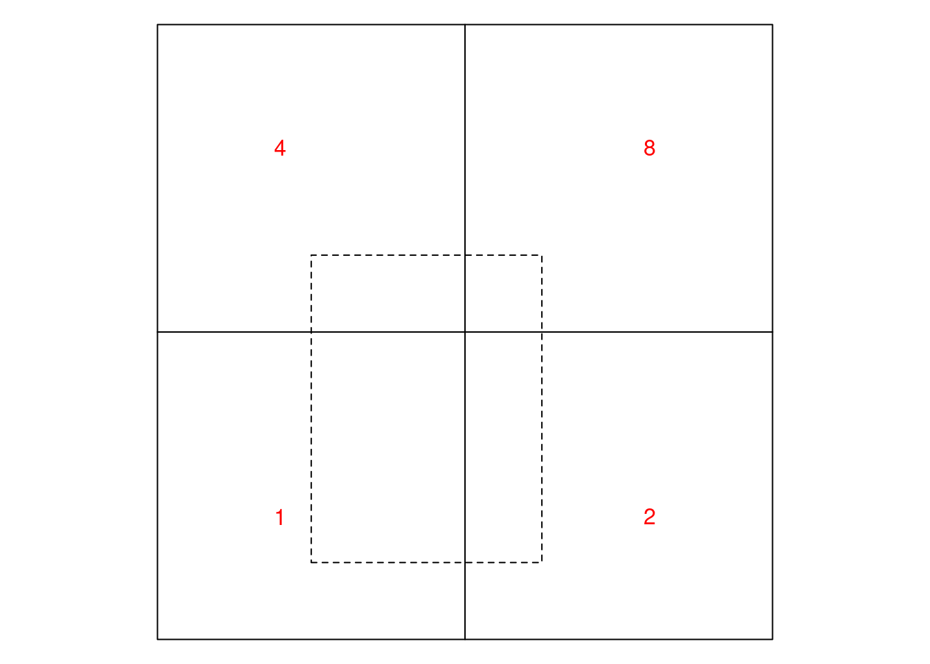
5. Consider @fig-awiex: using the equations in
@sec-extensiveintensive, compute the area-weighted interpolations
for (a) the dashed cell and (b) for the square enclosing all four solid
cells, first for the case where the four cells represent (i) an extensive
variable, and (ii) an intensive variable. The red numbers are the
data values of the source areas.
```{r fig-awiex, echo = !knitr::is_latex_output()}
#| out.width: 40%
#| fig.cap: "Example data for area-weighted interpolation"
#| code-fold: true
g <- st_make_grid(st_bbox(st_as_sfc("LINESTRING(0 0,1 1)")), n = c(2,2))
par(mar = rep(0,4))
plot(g)
plot(g[1] * diag(c(3/4, 1)) + c(0.25, 0.125), add = TRUE, lty = 2)
text(c(.2, .8, .2, .8), c(.2, .2, .8, .8), c(1,2,4,8), col = 'red')
```
<!--
* Find the name of the county that contains `POINT(-78.34046 35.017)`
* Find the names of all counties with boundaries that touch county `Sampson`.
* List the names of all counties that are less than 50 km away from county `Sampson`.
-->