How to load and save vector data in R
Summary:
If you have spatial vector data and are wondering how to load / save it in R, this tutorial is the answer to your questions. It presents practical examples for the most popular formats using the sf package. We will use free vector layers from Natural Earth as a data source.
Introduction
For convenience, all necessary files are located in the GitHub repository:
- countries.shp (and related files)
- rivers.gpkg
- cities.geojson
We can download the mentioned data and interactive notebook (.Rmd) manually from the repository (“Code” button > “Download ZIP”) or use the following script.
url = "https://github.com/kadyb/sf_load_save/archive/refs/heads/main.zip"
download.file(url, "sf_load_save.zip")
unzip("sf_load_save.zip")
In the first step, we need to download the sf package using the
install.packages() function, and then use the library() function to
load it into the session.
install.packages("sf")

library("sf")
Vector loading
Shapefile (.shp)
Let’s start by loading the shapefile format, which actually consists of several files (e.g., .shp, .shx, .dbf, .prj). More information can be found on Wikipedia, but currently it is not recommended to use this format due to its many limitations.
Generally, we can use the read_sf() function to load data. It requires
providing a path to the file. The file path can be defined in two ways
in R and this is the most common source of problems (errors like:
Error: Cannot open "file.shp"; The file doesn't seem to exist.).
The first way (easier) is to provide an absolute path, i.e. we must provide the exact location where the file is located. For instance:
path = "C:/Users/Krzysztof/Documents/file.shp"
However, this is
not
the recommended method, as it makes it impossible to locate files on
different operating systems. The second way is to specify a relative
path. In this case, we specify the location of the file relative to
the current working directory (or project). To find out where the
working directory is, we can use the getwd() function, and to change
it the setwd() function. For instance:
getwd()
#> "C:/Users/Krzysztof/Documents"
path = "file.shp"
Let’s load the shapefile using a relative path (all data can be found in
the data folder).
countries = read_sf("data/countries/countries.shp")
We can then print the metadata about this vector layer by referring to
the countries object.
countries

## Simple feature collection with 52 features and 168 fields
## Geometry type: MULTIPOLYGON
## Dimension:     XY
## Bounding box:  xmin: -17.53604 ymin: -34.82195 xmax: 51.41704 ymax: 37.3452
## Geodetic CRS:  WGS 84
## # A tibble: 52 × 169
##    featurecla   scalerank LABELRANK SOVEREIGNT SOV_A3 ADM0_DIF LEVEL TYPE  TLC
##    <chr>            <int>     <int> <chr>      <chr>     <int> <int> <chr> <chr>
##  1 Admin-0 cou…         0         2 Ethiopia   ETH           0     2 Sove… 1
##  2 Admin-0 cou…         0         3 South Sud… SDS           0     2 Sove… 1
##  3 Admin-0 cou…         0         6 Somalia    SOM           0     2 Sove… 1
##  4 Admin-0 cou…         0         2 Kenya      KEN           0     2 Sove… 1
##  5 Admin-0 cou…         0         6 Malawi     MWI           0     2 Sove… 1
##  6 Admin-0 cou…         0         3 United Re… TZA           0     2 Sove… 1
##  7 Admin-0 cou…         0         5 Somaliland SOL           0     2 Sove… 1
##  8 Admin-0 cou…         0         3 Morocco    MAR           0     2 Sove… 1
##  9 Admin-0 cou…         0         7 Western S… SAH           0     2 Inde… 1
## 10 Admin-0 cou…         0         4 Republic … COG           0     2 Sove… 1
## # ℹ 42 more rows
## # ℹ 160 more variables: ADMIN <chr>, ADM0_A3 <chr>, GEOU_DIF <int>,
## #   GEOUNIT <chr>, GU_A3 <chr>, SU_DIF <int>, SUBUNIT <chr>, SU_A3 <chr>,
## #   BRK_DIFF <int>, NAME <chr>, NAME_LONG <chr>, BRK_A3 <chr>, BRK_NAME <chr>,
## #   BRK_GROUP <chr>, ABBREV <chr>, POSTAL <chr>, FORMAL_EN <chr>,
## #   FORMAL_FR <chr>, NAME_CIAWF <chr>, NOTE_ADM0 <chr>, NOTE_BRK <chr>,
## #   NAME_SORT <chr>, NAME_ALT <chr>, MAPCOLOR7 <int>, MAPCOLOR8 <int>, …
We can see that this layer consists of 52 features (rows) and 168 fields (columns). The next information is about geometry type, dimension, spatial extent (bounding box) and coordinate reference system (CRS). In addition, the first 10 rows were printed.
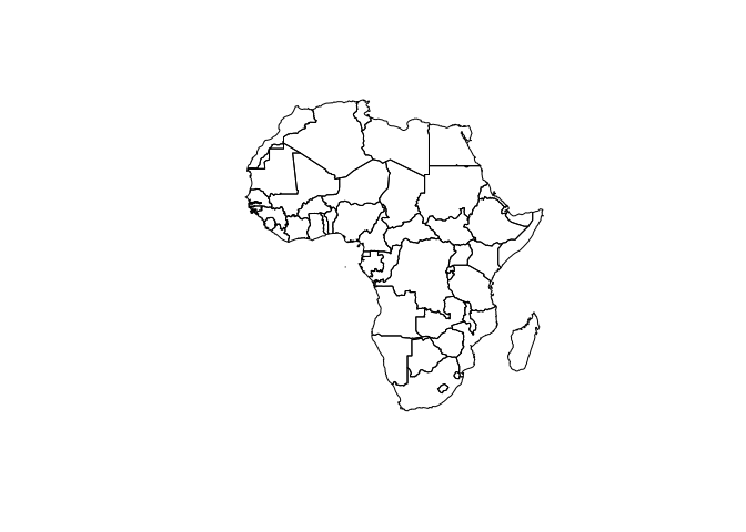
After loading the data, it is a good idea to present it on a map. A
simple plot() function can be used for this purpose. The countries
object has many fields (attributes), but to start with we only need
geometry. It can be obtained by using the st_geometry() function.
plot(st_geometry(countries))

GeoPackage (.gpkg)
The next dataset is rivers (linear geometry) saved in GeoPackage
format. It is loaded in exactly the same
way as the shapefile before. Note that this format can consist of
multiple layers of different types. In this case, we must define which
layer exactly we want to load. To check what layers are in the
geopackage, use the st_layers() function, and then specify it using
the layer argument in read_sf(). If the file only contains one
layer, we don’t need to do this.
st_layers("data/rivers.gpkg")

## Driver: GPKG
## Available layers:
##   layer_name     geometry_type features fields crs_name
## 1     rivers Multi Line String      228     38   WGS 84

rivers = read_sf("data/rivers.gpkg", layer = "rivers")
We can also display metadata as in the previous example.
rivers

## Simple feature collection with 228 features and 38 fields
## Geometry type: MULTILINESTRING
## Dimension:     XY
## Bounding box:  xmin: -16.54233 ymin: -34.34378 xmax: 49.46094 ymax: 35.12311
## Geodetic CRS:  WGS 84
## # A tibble: 228 × 39
##    dissolve  scalerank featurecla name  name_alt rivernum note  min_zoom name_en
##    <chr>         <int> <chr>      <chr> <chr>       <int> <chr>    <dbl> <chr>
##  1 975River          9 River      <NA>  <NA>          975 <NA>       7.1 <NA>
##  2 976River          9 River      Rung… <NA>          976 <NA>       7.1 Rungwa
##  3 977River          9 River      Ligo… <NA>          977 <NA>       7.1 Ligonha
##  4 978River          9 River      Dong… <NA>          978 <NA>       7.1 Dongwe
##  5 979River          9 River      Cuito <NA>          979 <NA>       7.1 Cuito
##  6 980Lake …         9 Lake Cent… <NA>  <NA>          980 <NA>       7.1 <NA>
##  7 980River          9 River      <NA>  <NA>          980 <NA>       7.1 <NA>
##  8 981River          9 River      Bagoé <NA>          981 <NA>       7.1 Bagoé
##  9 982River          9 River      Hade… <NA>          982 <NA>       7.1 Hadejia
## 10 983River          9 River      Sous  <NA>          983 <NA>       7.1 Sous
## # ℹ 218 more rows
## # ℹ 30 more variables: min_label <dbl>, ne_id <dbl>, label <chr>,
## #   wikidataid <chr>, name_ar <chr>, name_bn <chr>, name_de <chr>,
## #   name_es <chr>, name_fr <chr>, name_el <chr>, name_hi <chr>, name_hu <chr>,
## #   name_id <chr>, name_it <chr>, name_ja <chr>, name_ko <chr>, name_nl <chr>,
## #   name_pl <chr>, name_pt <chr>, name_ru <chr>, name_sv <chr>, name_tr <chr>,
## #   name_vi <chr>, name_zh <chr>, name_fa <chr>, name_he <chr>, …
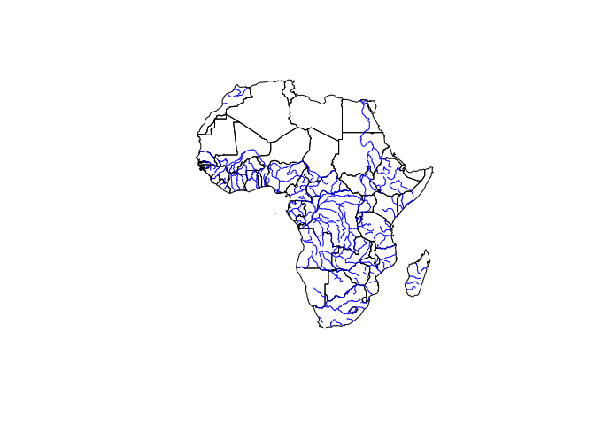
And make a visualization, but this time we will plot rivers against the
background of country borders. Adding more layers to the visualization
is done with the add = TRUE argument in plot() function. Note that
the order in which objects are added is important – the objects added
last are displayed at the top. The col argument is used to set the
color of the object.
plot(st_geometry(countries))
plot(st_geometry(rivers), add = TRUE, col = "blue")

GeoJSON (.geojson)
The last GeoJSON file contains cities in the world. In this case, we
also use the read_sf() function to load this file.
cities = read_sf("data/cities.geojson")
cities

## Simple feature collection with 1287 features and 31 fields
## Geometry type: POINT
## Dimension:     XY
## Bounding box:  xmin: -17.47508 ymin: -34.52953 xmax: 51.12333 ymax: 37.29042
## Geodetic CRS:  WGS 84
## # A tibble: 1,287 × 32
##    scalerank natscale labelrank featurecla      name   namepar namealt nameascii
##        <int>    <int>     <int> <chr>           <chr>  <chr>   <chr>   <chr>
##  1        10        1         8 Admin-1 capital Bassar <NA>    <NA>    Bassar
##  2        10        1         8 Admin-1 capital Sotou… <NA>    <NA>    Sotouboua
##  3        10        1         7 Admin-1 capital Meden… <NA>    <NA>    Medenine
##  4        10        1         7 Admin-1 capital Kebili <NA>    <NA>    Kebili
##  5        10        1         7 Admin-1 capital Tatao… <NA>    <NA>    Tataouine
##  6        10        1         7 Admin-1 capital L'Ari… <NA>    <NA>    L'Ariana
##  7        10        1         7 Admin-1 capital Jendo… <NA>    <NA>    Jendouba
##  8        10        1         7 Admin-1 capital Kasse… <NA>    <NA>    Kasserine
##  9        10        1         7 Admin-1 capital Sdid … <NA>    <NA>    Sdid Bou…
## 10        10        1         7 Admin-1 capital Silia… <NA>    <NA>    Siliana
## # ℹ 1,277 more rows
## # ℹ 24 more variables: adm0cap <int>, capalt <int>, capin <chr>,
## #   worldcity <int>, megacity <int>, sov0name <chr>, sov_a3 <chr>,
## #   adm0name <chr>, adm0_a3 <chr>, adm1name <chr>, iso_a2 <chr>, note <chr>,
## #   latitude <dbl>, longitude <dbl>, pop_max <int>, pop_min <int>,
## #   pop_other <int>, rank_max <int>, rank_min <int>, meganame <chr>,
## #   ls_name <chr>, min_zoom <dbl>, ne_id <int>, geometry <POINT [°]>
In this dataset, there is the featurecla column that indicates the
type of city. So let’s try to print them and then select only state
capitals.
We can print a column (attribute) in two ways, i.e. by specifying the column name in:
- Single square brackets – a spatial object will be printed
- Double square brackets (alternatively a dollar sign) – only the text will be printed
cities["featurecla"]

## Simple feature collection with 1287 features and 1 field
## Geometry type: POINT
## Dimension:     XY
## Bounding box:  xmin: -17.47508 ymin: -34.52953 xmax: 51.12333 ymax: 37.29042
## Geodetic CRS:  WGS 84
## # A tibble: 1,287 × 2
##    featurecla                  geometry
##    <chr>                    <POINT [°]>
##  1 Admin-1 capital    (0.7890036 9.261)
##  2 Admin-1 capital (0.9849965 8.557002)
##  3 Admin-1 capital       (10.4167 33.4)
##  4 Admin-1 capital     (8.971003 33.69)
##  5 Admin-1 capital         (10.4667 33)
##  6 Admin-1 capital      (10.2 36.86667)
##  7 Admin-1 capital      (8.749999 36.5)
##  8 Admin-1 capital   (8.716698 35.2167)
##  9 Admin-1 capital   (9.500004 35.0167)
## 10 Admin-1 capital   (9.383302 36.0833)
## # ℹ 1,277 more rows

# the `head()` function prints only the first 6 elements
head(cities[["featurecla"]])

## [1] "Admin-1 capital" "Admin-1 capital" "Admin-1 capital" "Admin-1 capital"
## [5] "Admin-1 capital" "Admin-1 capital"

# or alternatively
# head(cities$featurecla)
This layer contains 1287 different cities. To find out what types of
cities these are, we can use the table() function, which will
summarize them.
table(cities[["featurecla"]])

##
##        Admin-0 capital    Admin-0 capital alt        Admin-1 capital
##                     54                      6                    609
## Admin-1 region capital        Populated place
##                     19                    599
We are interested in Admin-0 capital and Admin-0 capital alt types
because some countries have two capitals. We make selection as follows
using the | (OR) operator:
sel = cities$featurecla == "Admin-0 capital" | cities$featurecla == "Admin-0 capital alt"
head(sel)

## [1] FALSE FALSE FALSE FALSE FALSE FALSE
As a result of this operation, we got a logical vector with TRUE and
FALSE values (if the city is / is not the capital). Now let’s create a
new object named capitals, which will contain only capitals.
# select only those cities that meet the above conditions
capitals = cities[sel, ]
capitals["name"]

## Simple feature collection with 60 features and 1 field
## Geometry type: POINT
## Dimension:     XY
## Bounding box:  xmin: -17.47508 ymin: -33.91807 xmax: 47.51468 ymax: 36.80278
## Geodetic CRS:  WGS 84
## # A tibble: 60 × 2
##    name                   geometry
##    <chr>               <POINT [°]>
##  1 Lobamba        (31.2 -26.46667)
##  2 Bir Lehlou (-9.652522 26.11917)
##  3 Kigali     (30.05859 -1.951644)
##  4 Mbabane    (31.13333 -26.31665)
##  5 Juba        (31.58003 4.829975)
##  6 Dodoma        (35.75 -6.183306)
##  7 Laayoune   (-13.20001 27.14998)
##  8 Djibouti      (43.148 11.59501)
##  9 Banjul      (-16.5917 13.45388)
## 10 Porto-Novo  (2.616626 6.483311)
## # ℹ 50 more rows
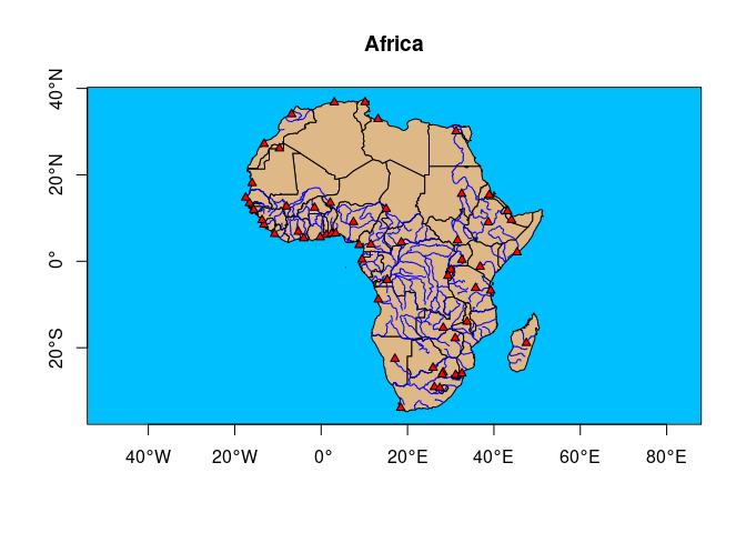
In the last step, we prepare the final visualization. We can add a title
(main argument), axes (axes argument) and change the background
color (bgc argument) of the figure. We can also change the point
symbol (pch argument), set its size (cex argument) and fill color
(bg argument).
plot(st_geometry(countries), main = "Africa", axes = TRUE, bgc = "deepskyblue",
     col = "burlywood")
plot(st_geometry(rivers), add = TRUE, col = "blue")
plot(st_geometry(capitals), add = TRUE, pch = 24, bg = "red", cex = 0.8)

Vector saving
Saving vector data is as easy as loading. There is a dedicated
write_sf() function for this purpose and it requires two arguments:
- The object we want to save
- The path to save with file extension
For example, let’s save our capital object as a GeoPackage (.gpkg),
but as an exercise you can save it in other formats as well (you just
need to change the extension).
write_sf(capitals, "data/capitals.gpkg")
Synopsis
The sf package allows loading vector data with the read_sf()
function and saving it with the write_sf() function in R. A list of
all supported vector formats can be found on the GDAL
website.
For more information, see:
- sf introductory vignette: Reading, Writing and Converting Simple Features
- Introduction to sf and stars in Spatial Data Science: With Applications in R (Pebesma E. & Bivand R., 2023)
Supplement
In the previous part of the tutorial, we looked at simple examples of loading vector data, while in this section we will check out more advanced ways.
Zipped shapefile (.shz)
As we noted earlier, a shapefile consists of several files, which can be
cumbersome. Some solution is to use zipped shapefiles, which is de facto
an archive. To create such a file, the extension .shz (or .shp.zip) and
the ESRI Shapefile driver are required. Loading is done in a standard
way by specifying the path to the “.shz” file.
write_sf(capitals, "data/capitals.shz", driver = "ESRI Shapefile")
Hooray, only one file on the disk!
Virtual File Systems
GDAL provides some facilities for loading files using some abstraction by Virtual File Systems. In practice, this means that we can refer directly to the files without first unpacking or downloading them in R. For example, we can directly open the shapefile that is in the archive on the website. To do this, we must use two prefixes:
/vsicurl/to download the file/vsizip/to unpack the archive
# URL is file path
url = "https://raw.githubusercontent.com/OSGeo/gdal/master/autotest/ogr/data/shp/poly.zip"
# note that the order of the prefixes is reverse
f = paste0("/vsizip/", "/vsicurl/", url)
read_sf(f)

## Simple feature collection with 10 features and 3 fields
## Geometry type: POLYGON
## Dimension:     XY
## Bounding box:  xmin: 478315.5 ymin: 4762880 xmax: 481645.3 ymax: 4765610
## Projected CRS: OSGB36 / British National Grid
## # A tibble: 10 × 4
##        AREA EAS_ID PRFEDEA                                              geometry
##       <dbl>  <dbl> <chr>                                           <POLYGON [m]>
##  1  215229.    168 35043411 ((479819.8 4765180, 479690.2 4765260, 479647 476537…
##  2  247328.    179 35043423 ((480035.3 4765558, 480039 4765540, 479730.4 476540…
##  3  261753.    171 35043414 ((479819.8 4765180, 479859.9 4765270, 479909.9 4765…
##  4  547597.    173 35043416 ((479014.9 4765148, 479029.7 4765110, 479117.8 4764…
##  5   15776.    172 35043415 ((479029.7 4765110, 479046.5 4765117, 479123.3 4765…
##  6  101430.    169 35043412 ((480083 4765050, 480080.3 4764980, 480134 4764856,…
##  7  268598.    166 35043409 ((480389.7 4764950, 480537.2 4765014, 480568 476491…
##  8 1634833.    158 35043369 ((480701.1 4764738, 480761.5 4764778, 480825 476482…
##  9  596610.    165 35043408 ((479750.7 4764702, 479968.5 4764788, 479985.1 4764…
## 10    5269.    170 35043413 ((479750.7 4764702, 479658.6 4764670, 479640.1 4764…
SQL preselection
We can use SQL queries to pre-filter features, so only selected objects / attributes will be loaded. This allows us to limit the size of the object in memory and speed up the operation time. Moreover, we can also make spatial selection, i.e. limit the loading of data only to a selected area.
Columns filtering
The query argument in the read_sf() function is used to pass SQL
queries. Let’s go back to the countries dataset and load only the
column with the names of countries (NAME_LONG).
sql = "SELECT NAME_LONG FROM countries"
f = "data/countries/countries.shp"
read_sf(f, query = sql)

## Simple feature collection with 52 features and 1 field
## Geometry type: MULTIPOLYGON
## Dimension:     XY
## Bounding box:  xmin: -17.53604 ymin: -34.82195 xmax: 51.41704 ymax: 37.3452
## Geodetic CRS:  WGS 84
## # A tibble: 52 × 2
##    NAME_LONG                                                            geometry
##    <chr>                                                      <MULTIPOLYGON [°]>
##  1 Ethiopia              (((34.0707 9.454592, 34.06689 9.531176, 34.09821 9.679…
##  2 South Sudan           (((35.92084 4.619332, 35.85654 4.619603, 35.78122 4.61…
##  3 Somalia               (((46.46696 6.538292, 46.48805 6.558645, 46.50841 6.57…
##  4 Kenya                 (((35.70585 4.619447, 35.70594 4.619962, 35.71152 4.66…
##  5 Malawi                (((34.96461 -11.57356, 34.65125 -11.57004, 34.61673 -1…
##  6 Tanzania              (((32.92086 -9.4079, 32.90546 -9.398185, 32.83074 -9.3…
##  7 Somaliland            (((48.93911 11.24913, 48.93911 11.13674, 48.93911 11.0…
##  8 Morocco               (((-8.817035 27.66146, -8.818449 27.6594, -8.81292 27.…
##  9 Western Sahara        (((-8.817035 27.66146, -8.816537 27.66147, -8.752562 2…
## 10 Republic of the Congo (((18.62639 3.476869, 18.63455 3.449222, 18.64241 3.32…
## # ℹ 42 more rows
Rows filtering
We can also select rows using a condition, e.g. population (POP_EST)
greater than 25 million.
sql = "SELECT * FROM countries WHERE POP_EST > 25000000"
f = "data/countries/countries.shp"
read_sf(f, query = sql) # 17 countries

## Simple feature collection with 17 features and 168 fields
## Geometry type: MULTIPOLYGON
## Dimension:     XY
## Bounding box:  xmin: -17.01374 ymin: -34.82195 xmax: 50.50392 ymax: 37.09394
## Geodetic CRS:  WGS 84
## # A tibble: 17 × 169
##    featurecla   scalerank LABELRANK SOVEREIGNT SOV_A3 ADM0_DIF LEVEL TYPE  TLC
##    <chr>            <int>     <int> <chr>      <chr>     <int> <int> <chr> <chr>
##  1 Admin-0 cou…         0         2 Ethiopia   ETH           0     2 Sove… 1
##  2 Admin-0 cou…         0         2 Kenya      KEN           0     2 Sove… 1
##  3 Admin-0 cou…         0         3 United Re… TZA           0     2 Sove… 1
##  4 Admin-0 cou…         0         3 Morocco    MAR           0     2 Sove… 1
##  5 Admin-0 cou…         0         2 Democrati… COD           0     2 Sove… 1
##  6 Admin-0 cou…         0         2 South Afr… ZAF           0     2 Sove… 1
##  7 Admin-0 cou…         0         3 Sudan      SDN           0     2 Sove… 1
##  8 Admin-0 cou…         0         3 Ivory Coa… CIV           0     2 Sove… 1
##  9 Admin-0 cou…         0         2 Nigeria    NGA           0     2 Sove… 1
## 10 Admin-0 cou…         0         3 Angola     AGO           0     2 Sove… 1
## 11 Admin-0 cou…         0         3 Algeria    DZA           0     2 Sove… 1
## 12 Admin-0 cou…         0         3 Mozambique MOZ           0     2 Sove… 1
## 13 Admin-0 cou…         0         3 Uganda     UGA           0     2 Sove… 1
## 14 Admin-0 cou…         0         3 Cameroon   CMR           0     2 Sove… 1
## 15 Admin-0 cou…         0         3 Ghana      GHA           0     2 Sove… 1
## 16 Admin-0 cou…         0         2 Egypt      EGY           0     2 Sove… 1
## 17 Admin-0 cou…         0         3 Madagascar MDG           0     2 Sove… 1
## # ℹ 160 more variables: ADMIN <chr>, ADM0_A3 <chr>, GEOU_DIF <int>,
## #   GEOUNIT <chr>, GU_A3 <chr>, SU_DIF <int>, SUBUNIT <chr>, SU_A3 <chr>,
## #   BRK_DIFF <int>, NAME <chr>, NAME_LONG <chr>, BRK_A3 <chr>, BRK_NAME <chr>,
## #   BRK_GROUP <chr>, ABBREV <chr>, POSTAL <chr>, FORMAL_EN <chr>,
## #   FORMAL_FR <chr>, NAME_CIAWF <chr>, NOTE_ADM0 <chr>, NOTE_BRK <chr>,
## #   NAME_SORT <chr>, NAME_ALT <chr>, MAPCOLOR7 <int>, MAPCOLOR8 <int>,
## #   MAPCOLOR9 <int>, MAPCOLOR13 <int>, POP_EST <dbl>, POP_RANK <int>, …
Spatial filtering
Finally, to perform spatial filtering, we must first define the spatial
extent / bounding box (st_bbox() function) and specify its coordinate
reference system (CRS). Then the bounding box needs to be converted into
a polygon using the st_as_sfc() function and finally converted to a
Well-Know
Text
representation using st_as_text() function. Therefore, prepared text
is passed to the wkt_filter argument. Follow the example below of
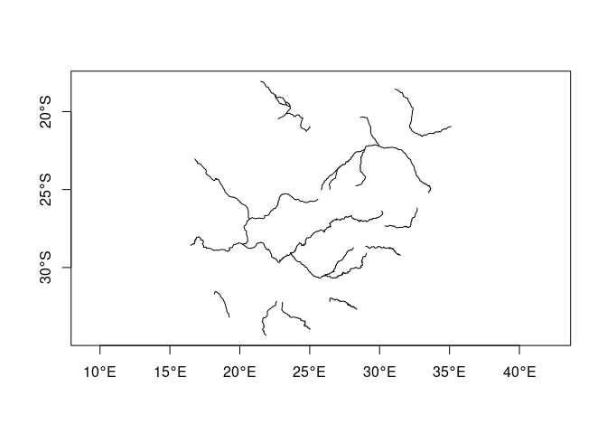
loading rivers only in southern Africa:
bbox = st_bbox(c(xmin = 10, xmax = 40, ymax = -35, ymin = -20),
               crs = st_crs(4326))
bbox = st_as_text(st_as_sfc(bbox))
bbox

## [1] "POLYGON ((10 -20, 40 -20, 40 -35, 10 -35, 10 -20))"

f = "data/rivers.gpkg"
rivers_south = read_sf(f, wkt_filter = bbox)
plot(st_geometry(rivers_south), axes = TRUE)

