Progress on R-spatial evolution, Apr 2023
spevolution status- Splitting
R_LIBS - ASDAR examples using
sforterra - Which
sforterramethods or functions match retiring methods or functions? - Conserving
spworkflows - Deprecation steps
- Moderate progress in de-coupling packages
- Reverse depencency checks 2023-03-22
Summary:
This is the third report on the R-spatial evolution project. The project
involves the retirement (archiving) of rgdal, rgeos and maptools
during 2023. The first
report set out the
main goals of the project. The second
report covered
progress so far, steps already taken, and those remaining to be
accomplished. A
talk
at the University of Chicago Center for Spatial Data Science in January
2023 has been made available as a
recording.
The talk is an intermediate report between the last blog and this blog,
and should be consulted for updates on topics not covered here
(including much better response to raising github issues for packages
compared to bulk emails).
There are now two key dates in the schedule:
-
during June 2023, in just three months, the internal evolution status setting of
spwill be changed from “business as usual” to “usesfinstead ofrgdalandrgeos. Packages depending onspmay need to addsfto their weak dependencies, and to monitor any changes in output. -
during October 2023, in seven months,
rgdal,rgeosandmaptoolswill be archived on CRAN, and packages with strong dependencies on the retiring packages must be either upgraded to usesf,terraor other alternatives or work-arounds by or before that time.
Waiting until October before acting risks workflow interruption, and is
not wise. A satisfying number of package maintainers with packages
depending on raster, which dropped rgdal and rgeos in favour of
terra six months ago, have already removed unneeded dependencies on
rgeos and rgdal. Making all required changes in the period from now
to the June sp change will mean just one round of adaptations rather
than two rounds.
In order to facilitate migration, this blog will present steps taken to
modify the sp, rgdal, rgeos and maptools code used in
ASDAR (Bivand, Pebesma, and Gomez-Rubio
2013), and to be found in this github
repository. This extends the
sf Wiki published
when sf was being introduced.
sp evolution status
Repeating from the second blog:
As mentioned in our first report, sp on CRAN has been provided with
conditional code that prevents sp calling most code in rgdal or
rgeos. This can be enabled before loading sp by setting e.g.:
options("sp_evolution_status"=2)
library(sp)
for checking packages under status
0: business as usual,1: stop ifrgdalorrgeosare absent, or2: usesfinstead ofrgdalandrgeos
or alternatively can be set as an environment variable read when sp is
loaded, e.g. when running checks from the command line by
_SP_EVOLUTION_STATUS_=2 R CMD check
This construction should permit maintainers to detect potential problems
in code. devtools::check() provides the env_vars= argument, which
may be used for the same purpose.
From sp 1.6.0 published on CRAN 2023-01-19, these status settings may
also be changed when sp is loaded, using sp::get_evolution_status()
returning the current value, and sp::set_evolution_status(value),
where value can take the integer values 0L, 1L and 2L.
Splitting R_LIBS
Maintainers may also find it helpful to split the user-writable package library into one main part, and a separate part containing only retiring packages. In this way one can detect other undocumented use of the retiring packages by mimicking the post-retirement scenario as installed retiring packages decay. In my case:
Sys.getenv("R_LIBS")

[1] "/home/rsb/lib/r_libs:/home/rsb/lib/r_libs_retiring"

(lP <- .libPaths())

[1] "/home/rsb/lib/r_libs"
[2] "/home/rsb/lib/r_libs_retiring"
[3] "/home/rsb/topics/R/R423-share/lib64/R/library"

length(r_libs <- list.files(lP[1]))

[1] 3982

(rets <- list.files(lP[2]))

[1] "maptools" "rgdal"    "rgeos"

rets %in% r_libs

[1] FALSE FALSE FALSE
This means that I can proceed without changing R_LIBS if I want loaded
packages to be able to see the installed retiring packages, but can
manipulate R_LIBS for example when checking:
_SP_EVOLUTION_STATUS_=2 R_LIBS="/home/rsb/lib/r_libs" R CMD check
to see that a package really avoids loading them.
The critical point will be reached in April 2024, when R 4.4 is
expected, and when the checkBuilt= argument to update.packages()
will show that the retiring packages are no longer available for the new
version of R. This can be emulated under control by splitting the
user-writable package library early.
ASDAR examples using sf or terra
The ASDAR (Bivand, Pebesma, and Gomez-Rubio 2013) examples use sp
evolution status and split R_LIBS extensively in nightly testing.
ASDAR code for both book editions has always been run nightly, to alert
the authors to anomalies from updates of packages and/or upstream
geospatial software libraries. The code in the sf_tests2ed repository
was based on the second edition code, updated and simplified. The files
for file comparison using diff and presented in HTML by diff2html
have been further cleaned, removing spurious differences introduced by
commenting out legacy code.
The results of file comparison by chapter are available through the
following links (all chapters using sf, chapters 2, 4 and 5 also using
terra in separate scripts):
Which sf or terra methods or functions match retiring methods or functions?
The ASDAR scripts give numerous examples of how use of functionality
from the retiring packages may be replaced by sf or terra and
coercion to or from sp classes. Using early March 2023 pkgapi runs
identifying CRAN packages using retiring package functions, line
references to the diffs for ch. 2, 4 and 5 have been added for sf and
terra variants, and lists of methods and functions from sf or
terra, in addition to lists of affected packages (also see:
https://github.com/r-spatial/evolution/blob/main/pkgapi_by_pkg_230305.csv).
The spreadsheet is wide, so scrolling right is required (or a wider
window):
https://github.com/r-spatial/evolution/blob/main/pkgapi_230305_refs.csv.
The main points are that rgeos binary predicates usually have similar
names in sf but in terra go through terra::relate, reading and
writing vector files are well-supported, reading and writing raster
files in terra::rast is more like the rgdal functions than through
stars, and so on.
These so far only cover functions called in code, not in examples or vignettes, but provide a good framework for required modifications.
Conserving sp workflows
While we encourage users and maintainers of packages currently utilising
the retiring packages to migrate fully to modern packages, such as
terra for raster users and sf and stars for other sp users,
some may prefer, in the short term, to keep sp workflows running, as
demonstrated in the ASDAR scripts. The diff files show that coercion
between representations is used extensively to mitigate the
non-availability of retiring packages. In the “Classes for Spatial Data”
chapter diffs, we see straight away that sp::CRS(), with rgdal
checking the CRS string, is replaced by as(sf::st_crs(), "CRS"), with
sf checking the CRS string. terra does not have a similar class, and
coordinate reference systems are part of instantiated objects or are
character strings.
rgrass has a
vignette
on spatial object coercion; rgrass uses terra for file transfer
between R and GRASS GIS, hence the examples start from object classes
defined in terra. The following is a short extract:
Sys.setenv("_SP_EVOLUTION_STATUS_"="2")
On loading and attaching, terra displays its version:
library("terra")

terra 1.7.18

library("sf")

Linking to GEOS 3.11.2, GDAL 3.6.3, PROJ 9.2.0; sf_use_s2() is TRUE

library("sp")

library("stars")

Loading required package: abind

library("raster")
terra::gdal() tells us the versions of the external libraries being
used by terra:
gdal(lib="all")

    gdal     proj     geos
 "3.6.3"  "9.2.0" "3.11.2"
"SpatVector" coercion
In the terra package (Hijmans 2023b), vector data are held in
"SpatVector" objects.
fv <- system.file("ex/lux.shp", package="terra")
(v <- vect(fv))

 class       : SpatVector
 geometry    : polygons
 dimensions  : 12, 6  (geometries, attributes)
 extent      : 5.74414, 6.528252, 49.44781, 50.18162  (xmin, xmax, ymin, ymax)
 source      : lux.shp
 coord. ref. : lon/lat WGS 84 (EPSG:4326)
 names       :  ID_1   NAME_1  ID_2   NAME_2  AREA   POP
 type        : <num>    <chr> <num>    <chr> <num> <int>
 values      :     1 Diekirch     1 Clervaux   312 18081
                   1 Diekirch     2 Diekirch   218 32543
                   1 Diekirch     3  Redange   259 18664
The coordinate reference system is expressed in WKT2-2019 form:
cat(crs(v), "\n")

GEOGCRS["WGS 84",
    DATUM["World Geodetic System 1984",
        ELLIPSOID["WGS 84",6378137,298.257223563,
            LENGTHUNIT["metre",1]]],
    PRIMEM["Greenwich",0,
        ANGLEUNIT["degree",0.0174532925199433]],
    CS[ellipsoidal,2],
        AXIS["geodetic latitude (Lat)",north,
            ORDER[1],
            ANGLEUNIT["degree",0.0174532925199433]],
        AXIS["geodetic longitude (Lon)",east,
            ORDER[2],
            ANGLEUNIT["degree",0.0174532925199433]],
    ID["EPSG",4326]]
"sf"
Most new work should use vector classes defined in the sf package
(Pebesma 2023, 2018), unless other terra classes are involved, in
which case the terra representation may be preferred. In this case,
coercion uses st_as_sf():
v_sf <- st_as_sf(v)
v_sf

Simple feature collection with 12 features and 6 fields
Geometry type: POLYGON
Dimension:     XY
Bounding box:  xmin: 5.74414 ymin: 49.44781 xmax: 6.528252 ymax: 50.18162
Geodetic CRS:  WGS 84
First 10 features:
   ID_1       NAME_1 ID_2           NAME_2 AREA    POP
1     1     Diekirch    1         Clervaux  312  18081
2     1     Diekirch    2         Diekirch  218  32543
3     1     Diekirch    3          Redange  259  18664
4     1     Diekirch    4          Vianden   76   5163
5     1     Diekirch    5            Wiltz  263  16735
6     2 Grevenmacher    6       Echternach  188  18899
7     2 Grevenmacher    7           Remich  129  22366
8     2 Grevenmacher   12     Grevenmacher  210  29828
9     3   Luxembourg    8         Capellen  185  48187
10    3   Luxembourg    9 Esch-sur-Alzette  251 176820
                         geometry
1  POLYGON ((6.026519 50.17767...
2  POLYGON ((6.178368 49.87682...
3  POLYGON ((5.881378 49.87015...
4  POLYGON ((6.131309 49.97256...
5  POLYGON ((5.977929 50.02602...
6  POLYGON ((6.385532 49.83703...
7  POLYGON ((6.316665 49.62337...
8  POLYGON ((6.425158 49.73164...
9  POLYGON ((5.998312 49.69992...
10 POLYGON ((6.039474 49.44826...
and the vect() method to get from sf to terra:
v_sf_rt <- vect(v_sf)
v_sf_rt

 class       : SpatVector
 geometry    : polygons
 dimensions  : 12, 6  (geometries, attributes)
 extent      : 5.74414, 6.528252, 49.44781, 50.18162  (xmin, xmax, ymin, ymax)
 coord. ref. : lon/lat WGS 84 (EPSG:4326)
 names       :  ID_1   NAME_1  ID_2   NAME_2  AREA   POP
 type        : <num>    <chr> <num>    <chr> <num> <int>
 values      :     1 Diekirch     1 Clervaux   312 18081
                   1 Diekirch     2 Diekirch   218 32543
                   1 Diekirch     3  Redange   259 18664

all.equal(v_sf_rt, v, check.attributes=FALSE)

[1] TRUE
"Spatial"
To coerce to and from vector classes defined in the sp package
(Bivand, Pebesma, and Gomez-Rubio 2013), methods in raster are used as
an intermediate step:
v_sp <- as(v, "Spatial")
print(summary(v_sp))

Object of class SpatialPolygonsDataFrame
Coordinates:
       min       max
x  5.74414  6.528252
y 49.44781 50.181622
Is projected: FALSE
proj4string : [+proj=longlat +datum=WGS84 +no_defs]
Data attributes:
      ID_1          NAME_1               ID_2          NAME_2
 Min.   :1.000   Length:12          Min.   : 1.00   Length:12
 1st Qu.:1.000   Class :character   1st Qu.: 3.75   Class :character
 Median :2.000   Mode  :character   Median : 6.50   Mode  :character
 Mean   :1.917                      Mean   : 6.50
 3rd Qu.:3.000                      3rd Qu.: 9.25
 Max.   :3.000                      Max.   :12.00
      AREA            POP
 Min.   : 76.0   Min.   :  5163
 1st Qu.:187.2   1st Qu.: 18518
 Median :225.5   Median : 26097
 Mean   :213.4   Mean   : 50167
 3rd Qu.:253.0   3rd Qu.: 36454
 Max.   :312.0   Max.   :182607

v_sp_rt <- vect(st_as_sf(v_sp))
all.equal(v_sp_rt, v, check.attributes=FALSE)

[1] TRUE
"SpatRaster" coercion
In the terra package, raster data are held in "SpatRaster" objects.
fr <- system.file("ex/elev.tif", package="terra")
(r <- rast(fr))

class       : SpatRaster
dimensions  : 90, 95, 1  (nrow, ncol, nlyr)
resolution  : 0.008333333, 0.008333333  (x, y)
extent      : 5.741667, 6.533333, 49.44167, 50.19167  (xmin, xmax, ymin, ymax)
coord. ref. : lon/lat WGS 84 (EPSG:4326)
source      : elev.tif
name        : elevation
min value   :       141
max value   :       547
In general, "SpatRaster" objects are files, rather than data held in
memory:
try(inMemory(r))

[1] FALSE
"stars"
The stars package (Pebesma 2022) uses GDAL through sf. A coercion
method is provided from "SpatRaster" to "stars":
r_stars <- st_as_stars(r)
print(r_stars)

stars object with 2 dimensions and 1 attribute
attribute(s):
          Min. 1st Qu. Median     Mean 3rd Qu. Max. NA's
elev.tif   141     291    333 348.3366     406  547 3942
dimension(s):
  from to  offset       delta refsys point x/y
x    1 95 5.74167  0.00833333 WGS 84 FALSE [x]
y    1 90 50.1917 -0.00833333 WGS 84 FALSE [y]
which round-trips in memory.
(r_stars_rt <- rast(r_stars))

class       : SpatRaster
dimensions  : 90, 95, 1  (nrow, ncol, nlyr)
resolution  : 0.008333333, 0.008333333  (x, y)
extent      : 5.741667, 6.533333, 49.44167, 50.19167  (xmin, xmax, ymin, ymax)
coord. ref. : lon/lat WGS 84 (EPSG:4326)
source(s)   : memory
name        : lyr.1
min value   :   141
max value   :   547
When coercing to "stars_proxy" the same applies:
(r_stars_p <- st_as_stars(r, proxy=TRUE))

stars_proxy object with 1 attribute in 1 file(s):
$elev.tif
[1] "[...]/elev.tif"

dimension(s):
  from to  offset       delta refsys point x/y
x    1 95 5.74167  0.00833333 WGS 84 FALSE [x]
y    1 90 50.1917 -0.00833333 WGS 84 FALSE [y]
with coercion from "stars_proxy" also not reading data into memory:
(r_stars_p_rt <- rast(r_stars_p))

class       : SpatRaster
dimensions  : 90, 95, 1  (nrow, ncol, nlyr)
resolution  : 0.008333333, 0.008333333  (x, y)
extent      : 5.741667, 6.533333, 49.44167, 50.19167  (xmin, xmax, ymin, ymax)
coord. ref. : lon/lat WGS 84 (EPSG:4326)
source      : elev.tif
name        : elevation
min value   :       141
max value   :       547
"RasterLayer"
From version 3.6-3 the raster package (Hijmans 2023a) uses terra for
all GDAL operations. Because of this, coercing a "SpatRaster" object
to a "RasterLayer" object is simple:
(r_RL <- raster(r))

class      : RasterLayer
dimensions : 90, 95, 8550  (nrow, ncol, ncell)
resolution : 0.008333333, 0.008333333  (x, y)
extent     : 5.741667, 6.533333, 49.44167, 50.19167  (xmin, xmax, ymin, ymax)
crs        : +proj=longlat +datum=WGS84 +no_defs
source     : elev.tif
names      : elevation
values     : 141, 547  (min, max)

inMemory(r_RL)

[1] FALSE
The WKT2-2019 CRS representation is present but not shown by default:
cat(wkt(r_RL), "\n")

GEOGCRS["unknown",
    DATUM["World Geodetic System 1984",
        ELLIPSOID["WGS 84",6378137,298.257223563,
            LENGTHUNIT["metre",1]],
        ID["EPSG",6326]],
    PRIMEM["Greenwich",0,
        ANGLEUNIT["degree",0.0174532925199433],
        ID["EPSG",8901]],
    CS[ellipsoidal,2],
        AXIS["longitude",east,
            ORDER[1],
            ANGLEUNIT["degree",0.0174532925199433,
                ID["EPSG",9122]]],
        AXIS["latitude",north,
            ORDER[2],
            ANGLEUNIT["degree",0.0174532925199433,
                ID["EPSG",9122]]]]
This object (held on file rather than in memory) can be round-tripped:
(r_RL_rt <- rast(r_RL))

class       : SpatRaster
dimensions  : 90, 95, 1  (nrow, ncol, nlyr)
resolution  : 0.008333333, 0.008333333  (x, y)
extent      : 5.741667, 6.533333, 49.44167, 50.19167  (xmin, xmax, ymin, ymax)
coord. ref. : +proj=longlat +datum=WGS84 +no_defs
source      : elev.tif
name        : elevation
min value   :       141
max value   :       547
"Spatial"
"RasterLayer" objects can be used for coercion from a "SpatRaster"
object to a "SpatialGridDataFrame" object:
r_sp_RL <- as(r_RL, "SpatialGridDataFrame")
summary(r_sp_RL)

Object of class SpatialGridDataFrame
Coordinates:
         min       max
s1  5.741667  6.533333
s2 49.441667 50.191667
Is projected: FALSE
proj4string : [+proj=longlat +datum=WGS84 +no_defs]
Grid attributes:
   cellcentre.offset    cellsize cells.dim
s1          5.745833 0.008333333        95
s2         49.445833 0.008333333        90
Data attributes:
   elevation
 Min.   :141.0
 1st Qu.:291.0
 Median :333.0
 Mean   :348.3
 3rd Qu.:406.0
 Max.   :547.0
 NA's   :3942
The WKT2-2019 CRS representation is present but not shown by default:
cat(wkt(r_sp_RL), "\n")

GEOGCRS["unknown",
    DATUM["World Geodetic System 1984",
        ELLIPSOID["WGS 84",6378137,298.257223563,
            LENGTHUNIT["metre",1]],
        ID["EPSG",6326]],
    PRIMEM["Greenwich",0,
        ANGLEUNIT["degree",0.0174532925199433],
        ID["EPSG",8901]],
    CS[ellipsoidal,2],
        AXIS["longitude",east,
            ORDER[1],
            ANGLEUNIT["degree",0.0174532925199433,
                ID["EPSG",9122]]],
        AXIS["latitude",north,
            ORDER[2],
            ANGLEUNIT["degree",0.0174532925199433,
                ID["EPSG",9122]]]]
This object can be round-tripped, but use of raster forefronts the
Proj.4 string CRS representation:
(r_sp_RL_rt <- raster(r_sp_RL))

class      : RasterLayer
dimensions : 90, 95, 8550  (nrow, ncol, ncell)
resolution : 0.008333333, 0.008333333  (x, y)
extent     : 5.741667, 6.533333, 49.44167, 50.19167  (xmin, xmax, ymin, ymax)
crs        : +proj=longlat +datum=WGS84 +no_defs
source     : memory
names      : elevation
values     : 141, 547  (min, max)

cat(wkt(r_sp_RL_rt), "\n")

GEOGCRS["unknown",
    DATUM["World Geodetic System 1984",
        ELLIPSOID["WGS 84",6378137,298.257223563,
            LENGTHUNIT["metre",1]],
        ID["EPSG",6326]],
    PRIMEM["Greenwich",0,
        ANGLEUNIT["degree",0.0174532925199433],
        ID["EPSG",8901]],
    CS[ellipsoidal,2],
        AXIS["longitude",east,
            ORDER[1],
            ANGLEUNIT["degree",0.0174532925199433,
                ID["EPSG",9122]]],
        AXIS["latitude",north,
            ORDER[2],
            ANGLEUNIT["degree",0.0174532925199433,
                ID["EPSG",9122]]]]

(r_sp_rt <- rast(r_sp_RL_rt))

class       : SpatRaster
dimensions  : 90, 95, 1  (nrow, ncol, nlyr)
resolution  : 0.008333333, 0.008333333  (x, y)
extent      : 5.741667, 6.533333, 49.44167, 50.19167  (xmin, xmax, ymin, ymax)
coord. ref. : +proj=longlat +datum=WGS84 +no_defs
source(s)   : memory
name        : elevation
min value   :       141
max value   :       547

crs(r_sp_RL_rt)

Coordinate Reference System:
Deprecated Proj.4 representation: +proj=longlat +datum=WGS84 +no_defs
WKT2 2019 representation:
GEOGCRS["unknown",
    DATUM["World Geodetic System 1984",
        ELLIPSOID["WGS 84",6378137,298.257223563,
            LENGTHUNIT["metre",1]],
        ID["EPSG",6326]],
    PRIMEM["Greenwich",0,
        ANGLEUNIT["degree",0.0174532925199433],
        ID["EPSG",8901]],
    CS[ellipsoidal,2],
        AXIS["longitude",east,
            ORDER[1],
            ANGLEUNIT["degree",0.0174532925199433,
                ID["EPSG",9122]]],
        AXIS["latitude",north,
            ORDER[2],
            ANGLEUNIT["degree",0.0174532925199433,
                ID["EPSG",9122]]]]
Coercion to the sp "SpatialGridDataFrame" representation is also
provided by stars:
r_sp_stars <- as(r_stars, "Spatial")
summary(r_sp_stars)

Object of class SpatialGridDataFrame
Coordinates:
        min       max
x  5.741667  6.533333
y 49.441667 50.191667
Is projected: FALSE
proj4string : [+proj=longlat +datum=WGS84 +no_defs]
Grid attributes:
  cellcentre.offset    cellsize cells.dim
x          5.745833 0.008333333        95
y         49.445833 0.008333333        90
Data attributes:
    elev.tif
 Min.   :141.0
 1st Qu.:291.0
 Median :333.0
 Mean   :348.3
 3rd Qu.:406.0
 Max.   :547.0
 NA's   :3942

cat(wkt(r_sp_stars), "\n")

GEOGCRS["WGS 84",
    ENSEMBLE["World Geodetic System 1984 ensemble",
        MEMBER["World Geodetic System 1984 (Transit)"],
        MEMBER["World Geodetic System 1984 (G730)"],
        MEMBER["World Geodetic System 1984 (G873)"],
        MEMBER["World Geodetic System 1984 (G1150)"],
        MEMBER["World Geodetic System 1984 (G1674)"],
        MEMBER["World Geodetic System 1984 (G1762)"],
        MEMBER["World Geodetic System 1984 (G2139)"],
        ELLIPSOID["WGS 84",6378137,298.257223563,
            LENGTHUNIT["metre",1]],
        ENSEMBLEACCURACY[2.0]],
    PRIMEM["Greenwich",0,
        ANGLEUNIT["degree",0.0174532925199433]],
    CS[ellipsoidal,2],
        AXIS["geodetic latitude (Lat)",north,
            ORDER[1],
            ANGLEUNIT["degree",0.0174532925199433]],
        AXIS["geodetic longitude (Lon)",east,
            ORDER[2],
            ANGLEUNIT["degree",0.0174532925199433]],
    USAGE[
        SCOPE["Horizontal component of 3D system."],
        AREA["World."],
        BBOX[-90,-180,90,180]],
    ID["EPSG",4326]]
and can be round-tripped:
(r_sp_stars_rt <- rast(st_as_stars(r_sp_stars)))

class       : SpatRaster
dimensions  : 90, 95, 1  (nrow, ncol, nlyr)
resolution  : 0.008333333, 0.008333333  (x, y)
extent      : 5.741667, 6.533333, 49.44167, 50.19167  (xmin, xmax, ymin, ymax)
coord. ref. : lon/lat WGS 84 (EPSG:4326)
source(s)   : memory
name        : lyr.1
min value   :   141
max value   :   547

cat(crs(r_sp_rt), "\n")

GEOGCRS["unknown",
    DATUM["World Geodetic System 1984",
        ELLIPSOID["WGS 84",6378137,298.257223563,
            LENGTHUNIT["metre",1]],
        ID["EPSG",6326]],
    PRIMEM["Greenwich",0,
        ANGLEUNIT["degree",0.0174532925199433],
        ID["EPSG",8901]],
    CS[ellipsoidal,2],
        AXIS["longitude",east,
            ORDER[1],
            ANGLEUNIT["degree",0.0174532925199433,
                ID["EPSG",9122]]],
        AXIS["latitude",north,
            ORDER[2],
            ANGLEUNIT["degree",0.0174532925199433,
                ID["EPSG",9122]]]]
Since spatial objects can be readily coerced between modern packages and
sp, input/output can be handled using the modern packages, making
rgdal redundant.
Deprecation steps
Functions and methods showing more usage from the pkgapi analysis in
the retiring packages are being deprecated. Deprecation uses the
.Deprecated() function in base R, which prints a message pointing to
alternatives and issuing a warning of class "deprecatedWarning".
rgdal >= 1.6-2, rgeos >= 0.6-1 and maptools >= 1.1-6 now
have larger numbers of such deprecation warnings. Deprecation warnings
do not lead to CRAN package check result warnings, so do not trigger
archiving notices from CRAN, but can and do trip up
testthat::expect_silent() and similar unit tests.
Moderate progress in de-coupling packages
There has been some progress in reducing package reverse dependency counts between January 2022 and early March 2023:
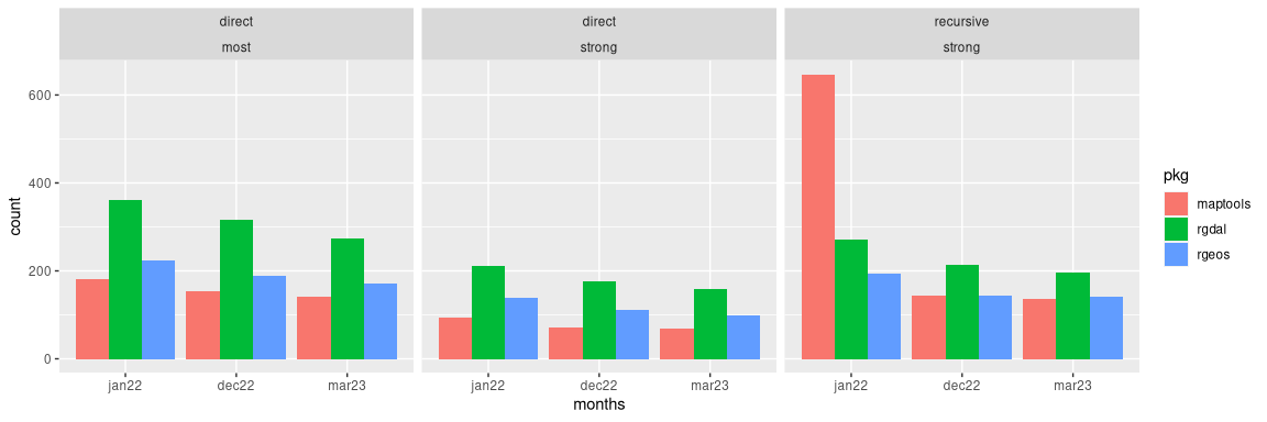 Some of the
 maptools recursive strong reduction are by archiving,
others as other popular packages like car have dropped maptools as a
strong dependency. maptools::pointLabel() is deprecated and is now
car::pointLabel() (and
https://github.com/sdray/adegraphics/issues/13), and adapted functions
based on these were deprecated as in
https://github.com/oscarperpinan/rastervis/issues/93. In addition,
almost 70 packages with strong dependencies on retiring packages through
raster in early 2023, now pass check without retiring packages on the
library path and sp evolution status 2L.
Reverse depencency checks 2023-03-22
Reverse dependency checks on CRAN and Bioconductor packages “most”
depending on retiring packages shows that 7 fail for sp evolution
status 2, of these some fail anyway. This implies that we can move to
shift sp evolution status default from 0 to 2 in June as planned.
Of the total of 729 packages checked, 293 fail with sp evolution
status 2 when the retiring packages are not on the library path. As
noted in the CSDS talk in mid-January, package maintainers contacted by
github issue seem to be much more responsive than other maintainers, so
work from April will concentrate on opening github issues for the 293
packages where possible, and adding to issues already opened, referring
to this document to give tips on how to migrate away from retiring
packages.
References
Bivand, Roger S., Edzer Pebesma, and Virgilio Gomez-Rubio. 2013. Applied Spatial Data Analysis with R, Second Edition. Springer, NY. https://asdar-book.org/.
Hijmans, Robert J. 2023a. raster: Geographic Data Analysis and Modeling. https://cran.r-project.org/package=raster.
———. 2023b. terra: Spatial Data Analysis. https://cran.r-project.org/package=terra.
Pebesma, Edzer. 2018. “Simple Features for R: Standardized Support for Spatial Vector Data.” The R Journal 10 (1): 439–46. https://doi.org/10.32614/RJ-2018-009.
———. 2022. stars: Spatiotemporal Arrays, Raster and Vector Data Cubes. https://CRAN.R-project.org/package=stars.
———. 2023. sf: Simple Features for R. https://cran.r-project.org/package=sf.