Processing large scale satellite imagery with openEO Platform and R
Summary: openEO is an open source, community-based API for cloud-based processing of Earth Observation data. This blog introduces the R openeo client, and demonstrates a sample analysis using the openEO Platform for processing.
openEO
OpenEO is an open source project that tries to make large-scale, cloud-based satellite image processing easier and more open. This blog post shows how the openEO client, available from CRAN and with online documentation here, can be used to explore datasets, compute on them, and download results.
From image collection to data cube
Image collections are collections of satellite images that are all processed in a uniform way. They are typically organized in tiles (or granules): raster files with all pixels obtained over an area observed in a single overpass of the satellite. Satellite image analysis often involves the analysis of a large number of tiles, obtained from different overpasses. The concept of data cubes makes it easier to analyse such data: a user defines the spatial extent and resolution, and the temporal extent and resolution, and all data is then reprocessed (aggregated) into the regular space and time resolutions. Cloud platforms such as openEO let the user define a data cube, and reprocess the data into this form before the final analysis steps are done. More explanation about datacubes in openEO is found here. The sample session below involves
- selecting an image collection, along with spatial and temporal extents
- selecting spectral bands
- reducing the spectral dimension by computing a single index
- aggregating the tiles to monthly median values
- downloading and plotting the resulting image time series
Sample session
An openEO session is started with loading the library, connecting to a back-end (here: openeo.cloud), and authenticating with the back-end:
library(openeo)
con = connect("openeo.cloud")
login()
The login will prompt for an authentication ID which can come from your organisation, or an openID-based mechanism such as google or GitHub. For loggin on you need an account on the back-end, as cloud computing in general is not a free resource. The openeo.cloud website has instructions on how to apply for a (ESA-) sponsored account with limited compute credits.
When these commands were carried out, and you are using RStudio as an IDE, RStudio will show an overview of the image collections available on this backend, which looks like this:
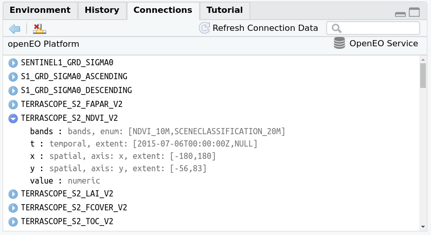
and which can help search for a particular collection. A more extensive viewer of the data collections is obtained in RStudio by
collection_viewer()
which opens a view window like this:
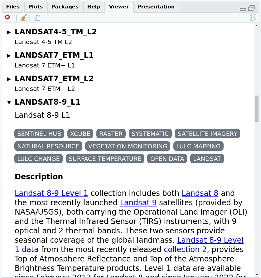
The same view is obtained online using this link. The set of image collections can also be obtained programmatically by
collections = list_collections(con)
names(collections) |> head()

## [1] "SENTINEL1_GRD_SIGMA0"     "S1_GRD_SIGMA0_ASCENDING"
## [3] "S1_GRD_SIGMA0_DESCENDING" "TERRASCOPE_S2_FAPAR_V2"
## [5] "TERRASCOPE_S2_NDVI_V2"    "TERRASCOPE_S2_LAI_V2"

length(collections)

## [1] 77
which can then be further processed in R.
We will work with Sentinel level 2A data, available in the collection
collection = "SENTINEL2_L2A"
coll_meta = describe_collection(collection)
names(coll_meta)

##  [1] "cube:dimensions" "description"     "extent"          "id"
##  [5] "keywords"        "license"         "links"           "providers"
##  [9] "stac_extensions" "stac_version"    "summaries"       "title"
information about the names and extents of data cube dimensions is for instance obtained by
coll_meta$`cube:dimensions`

## Dimension:    bands
## Type:         bands
## Values:       [B01,B02,B03,B04,B05,B06,B07,B08,B8A,B11,B12,SCL,relativeAzimuthAngles,sunZenithAngles,viewZenithAngles,B09,AOT,SNW,CLD,CLP,CLM,sunAzimuthAngles,viewAzimuthMean,viewZenithMean,dataMask]
##
## Dimension:    t
## Type:         temporal
## Extent:       [2015-07-06T00:00:00Z,NULL]
##
## Dimension:    x
## Type:         spatial
## Axis:         x
## Extent:       [-180,180]
##
## Dimension:    y
## Type:         spatial
## Axis:         y
## Extent:       [-56,83]
Next select a spatial region, a set of spectral bands and a time period to work on, by specifying a few R objects:
library(sf)

## Linking to GEOS 3.10.2, GDAL 3.4.3, PROJ 8.2.1; sf_use_s2() is TRUE

bbox = st_bbox(c(xmin = 7, xmax = 7.01, ymin = 52, ymax = 52.01), crs = 'EPSG:4326')
bands = c("B04", "B08")
time_range = list("2018-01-01", "2019-01-01")
We can then start building a process graph, the object that contains the work to be done on the back-end side. First we load the available processes from the back-end:
p = openeo::processes(con)
The object p now contains the processes available on the backend we
are using, and is used to define further tasks. We can explore the
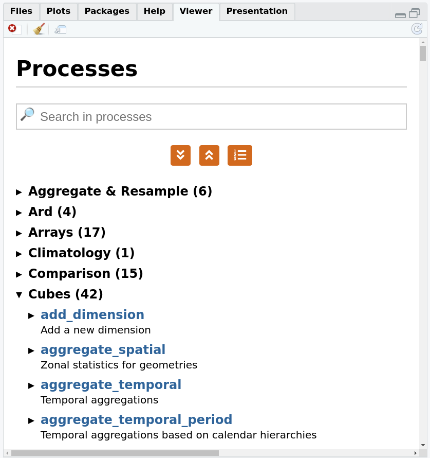
available processes by viewing them with
process_viewer()
which is shown below, or browse them online here.
We can constrain the image collection that we want to work on by its
name, extents in space and time, and bands (if no constraints are given,
the full extent is used). Using a member function of p here guarantees
that we do not use processes not available on the back-end:
data = p$load_collection(id = collection,
                         spatial_extent = bbox,
                         temporal_extent = time_range,
                         bands = bands)
We will compute NDVI, normalized differenced vegetation
index,
from the two selected bands, and use the NDVI function in
reduce_dimension to reduce dimension bands:
ndvi = function(data, context) {
  red = data[1]
  nir = data[2]
  (nir-red)/(nir+red)
}
calc_ndvi = p$reduce_dimension(data = data,
                               dimension = "bands",
                               reducer = ndvi)
Although ndvi is defined as an R function, in effect the openeo R
client translates this function into openEO native processes. This
cannot be done with arbitrarily complex functions, and passing on R
functions to be processed by an R instance in the back-end is done using
user-defined functions, the topic of a future blog post.
We will now process the NDVI values into a data cube with monthly
values, by picking for each pixel the median value of all pixels over
the month (Sentinel-2 has an image for roughly every 5 days). This is
done by aggregate_temporal_period:
temp_period = p$aggregate_temporal_period(data = calc_ndvi, period = "month",
                             reducer = function(data, context){p$median(data)},
                             dimension = "t")
Finally, we can define how we want to save results (which file format),
by the save_result process
result = p$save_result(data = temp_period, format="NetCDF")
and request the results synchronously by compute_results:
# synchronous:
compute_result(result, format = "NetCDF", output_file = "ndvi.nc", con = con)

## [1] "ndvi.nc"
All commands before compute_result() can be executed without
authentification; only compute_result asks for “real” computations on
imagery, and requires authentication, so that the compute costs can be
accounted for.
compute_result downloads the file locally, and we can now import it
and plot it either by e.g. ggplot2
library(stars)

## Loading required package: abind

r = read_stars("ndvi.nc")
library(ggplot2)
ggplot() + geom_stars(data = r) +
        facet_wrap(~t) + coord_equal() +
        theme_void() +
        scale_x_discrete(expand = c(0,0)) +
        scale_y_discrete(expand = c(0,0)) +
        scale_fill_viridis_c()
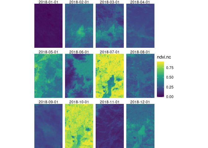
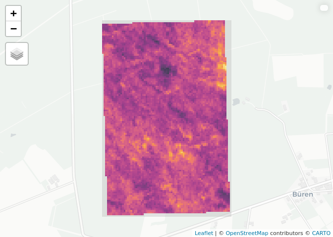
or by mapview (where the “real” mapview obviously gives an interactive
plot):
library(mapview)
mapview(r)
Batch jobs
The example above was deliberately kept very small; for larger jobs the
synchronous call to compute_result will time out, and a batch job can
be started with
job = create_job(graph = result, title = "ndvi.nc", description = "ndvi 2018")
start_job(job = job) # use the id of the job (job$id) to start the job
job_list = list_jobs() # here you can see all your jobs and their status
status(job)
The returned status is either queued, running, error or
finished. When it is finished, then results can be downloaded by
dwnld = download_results(job = job, folder = "./")
In case the status is error, error logs are obtained by
logs(job = job)
Further reading
The CRAN landing page has six (6!) vignettes on getting started, sample data retrieval, architecture, process graph building, and implementation details.
Upcoming…
The use of R functions that can be sent to the back-end and executed there by an R engine is under development. This is a big milestone, as it would provide arbitrary R functionality (given that arbitrary R packages would also be provided by the back-end), and is something that for instance Google Earth Engine can not provide. The current form in which this works is still a bit user-unfriendly (for the curious: examples are found in this repo, and contain still a mix of Python and R code). When this has been cleaned up and undergone more testing it will be the topic of a follow-up blog post.
