Reading Zarr files with R package stars

What is Zarr?
Aggregating global precipitation time series to countries
- 50m natural Earth country boundaries
simple aggregation
CMIP6 data
- Reading sub-arrays or strided arrays
- Using the classic GDAL raster API
Software versions

Summary: Zarr files are the new cloud native NetCDF, and are here to stay. This blog post will explore how they can be read in R using the GDAL “classic” raster API and the (relatively) new GDAL multidimensional array API, and how we can read sub-arrays or strided (subsampled, lower resolution) arrays. CMIP6 data is being released as Zarr data on the Google Cloud.

What is Zarr?

Zarr is a data format; it does not come in a single file as NetCDF or HDF5 does but as a directory with chunks of data in compressed files and metadata in JSON files. Zarr was developed in the Python numpy and xarray communities, and was quickly taken up by the Pangeo community. A Python-independent specification of Zarr (in progress, V3) is found here.

GDAL has a Zarr driver, and can read single (spatial, raster) slices without time reference through its classic raster API, and full time-referenced arrays through its newer multidimensional array API. In this blog post we show how these can be used through R and package stars for raster and vector data cubes. We will start with an attempt to reproduce what Ryan Abernathey did with Python, xarray and geopandas, published here.

Aggregating global precipitation time series to countries

Ryan’s blog post aggregates a global, 1-degree “square” gridded daily precipitation dataset (NASA GPCP) to country values, where the aggregation should be weighted according to the amount of overlap of grid cells (as “square” polygons) and country polygons.

We can read the rainfall data in R using

library(stars)
## Loading required package: abind
## Loading required package: sf
## Linking to GEOS 3.10.2, GDAL 3.4.3, PROJ 8.2.0; sf_use_s2() is TRUE
dsn = 'ZARR:"/vsicurl/https://ncsa.osn.xsede.org/Pangeo/pangeo-forge/gpcp-feedstock/gpcp.zarr"'
bounds = c(longitude = "lon_bounds", latitude = "lat_bounds")
r = read_mdim(dsn, bounds = bounds)
r
## stars object with 3 dimensions and 1 attribute
## attribute(s), summary of first 1e+05 cells:
##               Min. 1st Qu. Median   Mean  3rd Qu.     Max.
## precip [mm/d]    0       0      0 2.2841 1.618025 103.5965
## dimension(s):
##           from   to offset delta  refsys point                    values x/y
## longitude    1  360      0     1      NA    NA                      NULL [x]
## latitude     1  180    -90     1      NA    NA                      NULL [y]
## time         1 9226     NA    NA POSIXct    NA 1996-10-01,...,2021-12-31
st_bbox(r)
## xmin ymin xmax ymax 
##    0  -90  360   90
r[r < 0 | r > 100] = NA

where

the dsn is constructed such that GDAL knows this is a Zarr file (ZARR:) and that it is a web resource (/vsicurl/).
we specify the bounds because the latitude and longitude variables do not have a bounds attribute pointing to the cell boundaries, and their values do not point to grid cell centers (as recommended but not required by CF 1.10), but to boundaries
the Zarr has no CRS, so that R wouldn’t know these are ellipsoidal coordinates; without action it would then assume they are Cartesian coordinates (as geopandas does); we will correct this later on
values below 0 and above 100 are set to NA; this is according to the valid_range attribute for the precip variable, but not automatically parsed
time does not have an offset/delta pair, indicating it is not regular; there seem to be a few duplicate time steps, we can identify them by

time(r) |> diff() |> table()
## 
##     0 86400 
##     3  9222
ti = time(r)
ti[which(diff(ti) == 0)]
## [1] "2017-08-01 UTC" "2017-11-01 UTC" "2018-04-01 UTC"

50m natural Earth country boundaries

We can load the 50m NE Country boundaries from the rnaturalearth package:

library(rnaturalearth)
ne = ne_countries(scale = 50, returnclass = "sf")
st_crs(r) = st_crs(ne)
ne = st_make_valid(ne)

where

we set the CRS of the precipitation data cube, equal to that of NE (WGS84)
we call st_make_valid() to make the country boundaries valid on the sphere

simple aggregation

aggregate takes the grid cells as points:

(a = aggregate(r, ne, mean, na.rm = TRUE))
## stars object with 2 dimensions and 1 attribute
## attribute(s), summary of first 1e+05 cells:
##               Min.      1st Qu.    Median     Mean  3rd Qu.     Max.  NA's
## precip [mm/d]    0 3.206655e-05 0.5487042 2.849516 3.355176 97.14838 28631
## dimension(s):
##          from   to offset delta                       refsys point
## geometry    1  241     NA    NA +proj=longlat +datum=WGS8... FALSE
## time        1 9226     NA    NA                      POSIXct    NA
##                                                                     values
## geometry MULTIPOLYGON (((-69.91182 1...,...,MULTIPOLYGON (((31.42949 -2...
## time                                             1996-10-01,...,2021-12-31

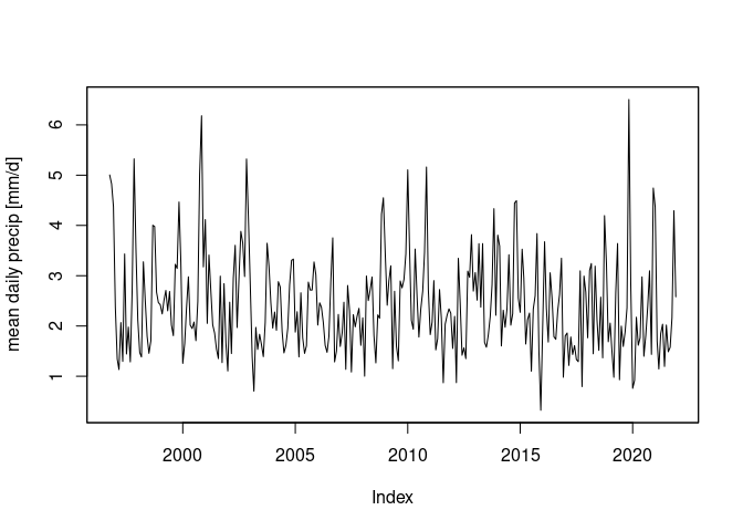
and returns a vector data cube: an array with 241 country geometries x 9226 time steps (days). We can select the time series for Italy and plot it, using the time series package xts, and aggregation to monthly mean values from xts:

library(xts)
## Loading required package: zoo
## 
## Attaching package: 'zoo'
## The following objects are masked from 'package:base':
## 
##     as.Date, as.Date.numeric
a[, which(ne$admin == "Italy"),] |>  # select Italy
    adrop() |>  # drop geometry dimension
    as.xts() -> a.xts # convert to xts (time series class)
a.xts |>
    aggregate(as.Date(cut(time(a.xts), "month")), mean, na.rm = TRUE) |> # temporal aggregation
    plot(ylab = "mean daily precip [mm/d]")

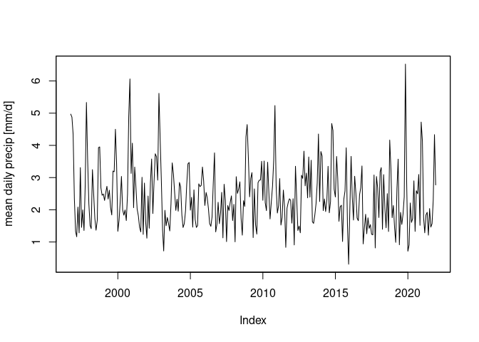
The “exact” (or “conservative region”) aggregation in Ryan’s blog is obtained by area-weighted interpolation; we have s2 on to get intersection using spherical coordinates; doing this with Cartesian coordinates will not work for half of the globe unless we’d recenter the precipitation coordinates from [0,360] to [-180,180]:

sf_use_s2() # the default
## [1] TRUE
ne = st_make_valid(ne)
it = ne[ne$admin == "Italy",]
st_interpolate_aw(r, it, extensive = FALSE) |>
    st_set_dimensions("time", time(r)) -> a2
## Warning in st_interpolate_aw.sf(st_as_sf(x), to, extensive, ...):
## st_interpolate_aw assumes attributes are constant or uniform over areas of x
a2 |> 
    adrop() |> 
    as.xts() |>
    aggregate(as.Date(cut(time(a2), "month")), mean, na.rm = TRUE) |> # monthly means
    plot(ylab = "mean daily precip [mm/d]")

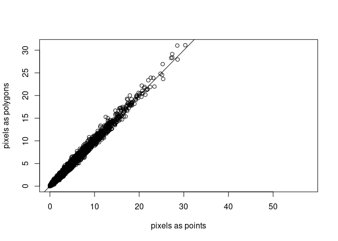
We can compare outcomes from both computations e.g. in a scatter plot:

a2 |> adrop() |> as.xts() -> a2.xts
plot(as.vector(a.xts), as.vector(a2.xts),
     xlab = "pixels as points", ylab = "pixels as polygons")
abline(0, 1)

CMIP6 data

CMIP6, the climate model intercomparison project, will share its output data (simulations of climate projections) as NetCDF but also as Zarr files on Google Cloud Storage. A STAC interface (static) to these data is found here.

One of these files, containing pressure at sea level for 6-hour intervals, was created by the following Python script:

import fsspec
import xarray
import zarr
m = fsspec.get_mapper("https://storage.googleapis.com/cmip6/CMIP6/HighResMIP/CMCC/CMCC-CM2-HR4/highresSST-present/r1i1p1f1/6hrPlev/psl/gn/v20170706")
ds = xarray.open_zarr(m)
ds.sel(time=slice("1948-01-01","1955-12-31")).to_zarr("./psl.zarr")

That file is provided here, but we will read the same file directly from the cloud storage using R:

dsn = 'ZARR:"/vsicurl/https://storage.googleapis.com/cmip6/CMIP6/HighResMIP/CMCC/CMCC-CM2-HR4/highresSST-present/r1i1p1f1/6hrPlev/psl/gn/v20170706"/:psl.zarr/'
d = read_mdim(dsn, count = c(NA, NA, 11680))
st_crs(d) = 'OGC:CRS84'
d
## stars object with 3 dimensions and 1 attribute
## attribute(s), summary of first 1e+05 cells:
##              Min. 1st Qu.   Median     Mean  3rd Qu.     Max.
## psl [Pa] 95056.82 99547.8 100975.1 100752.8 101700.6 105274.6
## dimension(s):
##      from    to     offset   delta    refsys point
## lon     1   288     -0.625    1.25    WGS 84    NA
## lat     1   192         NA      NA    WGS 84    NA
## time    1 11680 1948-01-01 6 hours PCICt_365    NA
##                               values x/y
## lon                             NULL [x]
## lat  [-90,-89.5288),...,[89.5288,90) [y]
## time                            NULL
st_bbox(d)
##    xmin    ymin    xmax    ymax 
##  -0.625 -90.000 359.375  90.000

where:

in addition to the ZARR: and /vsicurl/ prefixes, we see the array name (psl.zarr) specified
the count for time, corresponding to the time slices, is given, leaving the ones for longitude and latitude to NA
dimension information can be obtained using the gdalmdiminfo binary, or from R using

ret = gdal_utils("mdiminfo", dsn, quiet = TRUE)
jsonlite::fromJSON(ret)$dimensions
##   name full_name  size         type direction indexing_variable
## 1 bnds     /bnds     2         <NA>      <NA>              <NA>
## 2  lat      /lat   192 HORIZONTAL_Y     NORTH              /lat
## 3  lon      /lon   288 HORIZONTAL_X      EAST              /lon
## 4 time     /time 97820     TEMPORAL      <NA>             /time

bounds are being read, and as they are specified as an attribute to the coordinate variables:

jsonlite::fromJSON(ret)$arrays$lon$attributes$bounds
## [1] "lon_bnds"
jsonlite::fromJSON(ret)$arrays$lat$attributes$bounds
## [1] "lat_bnds"

we can see from the print summary that the latitude bounds are irregular: the ones touching the poles are half the latitude width as all others. Reading this as a regular GDAL file creates problems.
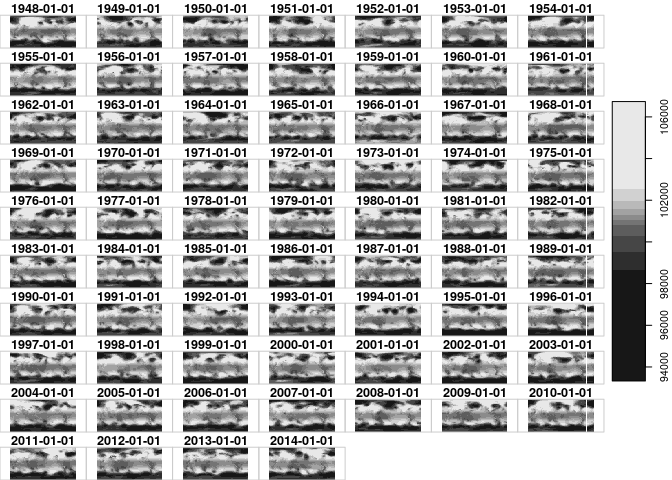
we also see is the the refsys (reference system) of the time is PCICt_365, indicating a “365-day” calendar is used: leap days are ignored.

A regular sequence of 6-hour images is provided for the non-leap days. Using package PCICt we can convert this to POSIXct time (the one we live in) by

as.POSIXct(r)
## stars object with 3 dimensions and 1 attribute
## attribute(s), summary of first 1e+05 cells:
##               Min. 1st Qu. Median     Mean  3rd Qu.     Max. NA's
## precip [mm/d]    0       0      0 2.283087 1.617958 99.58805    1
## dimension(s):
##           from   to offset delta                       refsys point
## longitude    1  360      0     1 +proj=longlat +datum=WGS8...    NA
## latitude     1  180    -90     1 +proj=longlat +datum=WGS8...    NA
## time         1 9226     NA    NA                      POSIXct    NA
##                              values x/y
## longitude                      NULL [x]
## latitude                       NULL [y]
## time      1996-10-01,...,2021-12-31

after which we see that we no longer have a regular time dimension but semi-regular with gaps (the leap days); POSIXct values are now in the values field of the time dimension.

We can plot the first 49 time slices e.g. by

plot(r[,,,1:49]) # first 49 time steps
## downsample set to 2

Reading sub-arrays or strided arrays

Using the multidimensional array API we can read lower reslution versions of the imagery by setting

offset the offset (start) of reading (pixels, 0, 0, 0 by default)
count the number of steps to read in each dimensions
step the step size in each dimension

As an example, let’s try to read one value per year:

(r = read_mdim(dsn, step = c(1, 1, 365 * 4)))
## stars object with 3 dimensions and 1 attribute
## attribute(s), summary of first 1e+05 cells:
##              Min.  1st Qu.   Median     Mean  3rd Qu.     Max.
## psl [Pa] 94926.56 99828.71 101017.5 100794.7 101698.9 105274.6
## dimension(s):
##      from  to     offset    delta    refsys point
## lon     1 288     -0.625     1.25        NA    NA
## lat     1 192         NA       NA        NA    NA
## time    1  67 1948-01-01 365 days PCICt_365    NA
##                               values x/y
## lon                             NULL [x]
## lat  [-90,-89.5288),...,[89.5288,90) [y]
## time                            NULL
plot(r)
## downsample set to 2

We can for instance read yearly data at a quarter of the spatial resolution by

(r = read_mdim(dsn, step = c(4, 4, 365 * 4)))
## stars object with 3 dimensions and 1 attribute
## attribute(s):
##              Min.  1st Qu. Median     Mean  3rd Qu.   Max.
## psl [Pa] 93488.44 99865.04 101041 100815.3 101760.1 106605
## dimension(s):
##      from to     offset    delta    refsys point
## lon     1 72       -2.5        5        NA    NA
## lat     1 48         NA       NA        NA    NA
## time    1 67 1948-01-01 365 days PCICt_365    NA
##                                      values x/y
## lon                                    NULL [x]
## lat  [-90,-89.5288),...,[86.70157,87.64398) [y]
## time                                   NULL
plot(r)

Using the classic GDAL raster API

We can explore the the zarr file by omitting the array name, e.g. by

dsn = 'ZARR:"/vsicurl/https://storage.googleapis.com/cmip6/CMIP6/HighResMIP/CMCC/CMCC-CM2-HR4/highresSST-present/r1i1p1f1/6hrPlev/psl/gn/v20170706"/'
gdal_utils("info", dsn)
## Driver: Zarr/Zarr
## Files: none associated
## Size is 512, 512
## Subdatasets:
##   SUBDATASET_1_NAME=ZARR:"/vsicurl/https://storage.googleapis.com/cmip6/CMIP6/HighResMIP/CMCC/CMCC-CM2-HR4/highresSST-present/r1i1p1f1/6hrPlev/psl/gn/v20170706/":/lat
##   SUBDATASET_1_DESC=Array /lat
##   SUBDATASET_2_NAME=ZARR:"/vsicurl/https://storage.googleapis.com/cmip6/CMIP6/HighResMIP/CMCC/CMCC-CM2-HR4/highresSST-present/r1i1p1f1/6hrPlev/psl/gn/v20170706/":/lon
##   SUBDATASET_2_DESC=Array /lon
##   SUBDATASET_3_NAME=ZARR:"/vsicurl/https://storage.googleapis.com/cmip6/CMIP6/HighResMIP/CMCC/CMCC-CM2-HR4/highresSST-present/r1i1p1f1/6hrPlev/psl/gn/v20170706/":/time
##   SUBDATASET_3_DESC=Array /time
##   SUBDATASET_4_NAME=ZARR:"/vsicurl/https://storage.googleapis.com/cmip6/CMIP6/HighResMIP/CMCC/CMCC-CM2-HR4/highresSST-present/r1i1p1f1/6hrPlev/psl/gn/v20170706/":/lat_bnds
##   SUBDATASET_4_DESC=Array /lat_bnds
##   SUBDATASET_5_NAME=ZARR:"/vsicurl/https://storage.googleapis.com/cmip6/CMIP6/HighResMIP/CMCC/CMCC-CM2-HR4/highresSST-present/r1i1p1f1/6hrPlev/psl/gn/v20170706/":/lon_bnds
##   SUBDATASET_5_DESC=Array /lon_bnds
##   SUBDATASET_6_NAME=ZARR:"/vsicurl/https://storage.googleapis.com/cmip6/CMIP6/HighResMIP/CMCC/CMCC-CM2-HR4/highresSST-present/r1i1p1f1/6hrPlev/psl/gn/v20170706/":/psl
##   SUBDATASET_6_DESC=Array /psl
##   SUBDATASET_7_NAME=ZARR:"/vsicurl/https://storage.googleapis.com/cmip6/CMIP6/HighResMIP/CMCC/CMCC-CM2-HR4/highresSST-present/r1i1p1f1/6hrPlev/psl/gn/v20170706/":/time_bnds
##   SUBDATASET_7_DESC=Array /time_bnds
## Corner Coordinates:
## Upper Left  (    0.0,    0.0)
## Lower Left  (    0.0,  512.0)
## Upper Right (  512.0,    0.0)
## Lower Right (  512.0,  512.0)
## Center      (  256.0,  256.0)

which lists the subdatasets; if we would ask for info on a subdatasetname we see an error:

dsn = 'ZARR:"/vsicurl/https://storage.googleapis.com/cmip6/CMIP6/HighResMIP/CMCC/CMCC-CM2-HR4/highresSST-present/r1i1p1f1/6hrPlev/psl/gn/v20170706/":/psl'
gdal_utils("info", dsn)
## Warning in CPL_gdalinfo(if (missing(source)) character(0) else source,
## options, : GDAL Error 1: Indices of extra dimensions must be specified

indicating that we need to add an index of the additional dimension (time). If we add e.g. index 10, we get

dsn = 'ZARR:"/vsicurl/https://storage.googleapis.com/cmip6/CMIP6/HighResMIP/CMCC/CMCC-CM2-HR4/highresSST-present/r1i1p1f1/6hrPlev/psl/gn/v20170706/":/psl:10'
gdal_utils("info", dsn)
## Driver: Zarr/Zarr
## Files: none associated
## Size is 288, 192
## Origin = (-0.625000000000000,-90.471204188481678)
## Pixel Size = (1.250000000000000,0.942408376963351)
## Metadata:
##   cell_measures=area: areacella
##   cell_methods=area: time: mean
##   comment=Sea Level Pressure
##   long_name=Sea Level Pressure
##   standard_name=air_pressure_at_sea_level
## Corner Coordinates:
## Upper Left  (  -0.6250000, -90.4712042) 
## Lower Left  (  -0.6250000,  90.4712042) 
## Upper Right (     359.375,     -90.471) 
## Lower Right (     359.375,      90.471) 
## Center      ( 179.3750000,   0.0000000) 
## Band 1 Block=288x192 Type=Float32, ColorInterp=Undefined
##   NoData Value=1.00000002004087734e+20
##   Unit Type: Pa

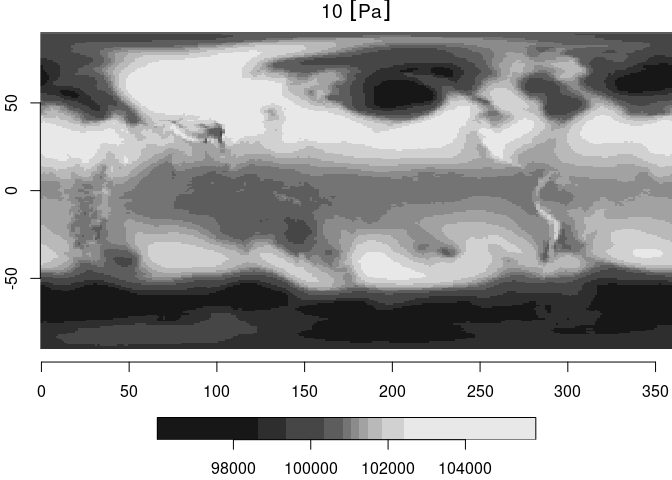
which describes a 288 x 192 pixel raster layer. It also reveals that GDAL thinks that this raster file has latitude dimensions exceeding [-90,90]. We can read such a slice with read_stars and plot the result:

(r0 = read_stars(dsn))
## stars object with 2 dimensions and 1 attribute
## attribute(s):
##             Min.  1st Qu.   Median     Mean  3rd Qu.     Max.
## 10 [Pa] 96032.01 99854.94 101043.6 100784.3 101660.2 105820.4
## dimension(s):
##   from  to   offset    delta refsys point values x/y
## x    1 288   -0.625     1.25     NA    NA   NULL [x]
## y    1 192 -90.4712 0.942408     NA    NA   NULL [y]
plot(r0, axes = TRUE)

Software versions

To use the features in this blog post for reading sub-arrays or lower resolution arrays, you need stars >= 0.5-7 and sf >= 1.0-9, which you can get by installing from source by

remotes::install_github("r-spatial/sf") # requires rtools42 on windows
remotes::install_github("r-spatial/stars")

You need both, since stars uses sf’s binding to GDAL - stars is a pure R package, all linking to GDAL happens through sf.

Alternatively, and in particular if you use Windows or MACOS you could install the github versions as binary package from r-universe:

install.packages("sf", repos = "https://r-spatial.r-universe.dev")
install.packages("stars", repos = "https://r-spatial.r-universe.dev")

update users have reported failure to reproduce the steps in this blog post. Note that this blog post was run on a version of sf linked to GDAL 3.4.3 from the ubuntugis-unstable ppa. If you have sf linked to an older version of GDAL, or if the GDAL version was not linked against BLOSC, then this (or parts of it) may not work. Note that Zarr, and Zarr support in GDAL are all very recent developments, and it takes time for modern library support to propagate through e.g. CRAN build toolchains – we are working on it!