Which gap does the sftime package fill?
A motivating example
- Geometrical operations and subsetting
- Plotting
Another motivating example: earthquake events
The sftime class
- Object structure
- Conversion from and to sftime
Available methods
Outlook

We are glad to report on the first CRAN release of the sftime package. The aim of sftime is to extent simple features from the sf package to handle (irregular) spatiotemporal data, such as records on earthquakes, accidents, disease or death cases, lightning strikes, data from weather stations, but also movement data which have further constraints.

This blog post

explains what gap the sftime package intents to fill,
provides two motivating examples to show how sftime objects can be used,
introduces the format of the sftime class, conversion methods from and to other classes, and available methods for class sftime,
and gives an outlook to the planned integration with gstat and spcopula to support spatiotemporal statistical analyses and future developments of sftime.

Which gap does the `sftime` package fill?

The stars package is an extension to sf which already handles regular spatiotemporal data — data cubes with spatial and regular temporal dimensions — such as gridded temperature values (raster time series) and vector data with temporal records at regular temporal instances (e.g. election results in states). From a historical perspective, stars objects replaced the STF and STS classes in the spacetime package.

What stars cannot handle are simple features where the spatial and temporal dimension are irregular. Irregular spatiotemporal data often arise in research and other applications, for example when analyzing aforementioned cases of earthquakes, accidents, disease or death cases, lightning strikes, data from weather stations, and movement data. From a historical perspective, sftime is intended to replace the STI and STT (trajectory data) classes in the spacetime package (in company of more specialized packages for trajectory data, such as sftrack).

Even though sftime can in principle also handle regular spatiotemporal data, stars is the preferred option to handle such data — sftime is not focused on regular spatiotemporal data. Thus, sftime complements the capabilities of the stars package for irregular spatiotemporal data.

A motivating example

Here, we:

provide a first glimpse on the sftime class,
show one way to create an sftime object from an sf object, and
show some visualization possibilities for sftime objects.

To this end, we directly build on top of the Tidy storm trajectories blog post which uses the storm trajectory data from the dplyr package — a perfect example for irregular spatiotemporal data.

First, we need to prepare the data and convert it into an sf object as described in the blog post:

# packages
library(dplyr)
#> 
#> Attaching package: 'dplyr'
#> The following object is masked from 'package:kableExtra':
#> 
#>     group_rows
#> The following objects are masked from 'package:stats':
#> 
#>     filter, lag
#> The following objects are masked from 'package:base':
#> 
#>     intersect, setdiff, setequal, union
library(sf)
#> Linking to GEOS 3.10.1, GDAL 3.4.0, PROJ 8.2.0; sf_use_s2() is TRUE
library(sftime)
library(rnaturalearth)

# convert to sf object
storms_sf <- 
  storms %>% 
  st_as_sf(coords = c("long", "lat"), crs = 4326) %>% 
  mutate(
    time = 
      paste(paste(year, month, day, sep = "-"), paste(hour, ":00", sep = "")) %>%
      as.POSIXct()
  ) %>% 
  select(-month, -day, -hour)

Now, sftime comes into play:

library(sftime)

# convert to sftime object
storms_sftime <- st_as_sftime(storms_sf)

storms_sftime
#> Spatiotemporal feature collection with 10010 features and 8 fields
#> Geometry type: POINT
#> Dimension:     XY
#> Bounding box:  xmin: -109.3 ymin: 7.2 xmax: -6 ymax: 51.9
#> Geodetic CRS:  WGS 84
#> Time column with class: 'POSIXt'.
#> Ranging from 1975-06-27 to 2015-11-11 18:00:00.
#> # A tibble: 10,010 × 10
#>    name   year status            category  wind pressure ts_diameter hu_diameter
#>  * <chr> <dbl> <chr>             <ord>    <int>    <int>       <dbl>       <dbl>
#>  1 Amy    1975 tropical depress… -1          25     1013          NA          NA
#>  2 Amy    1975 tropical depress… -1          25     1013          NA          NA
#>  3 Amy    1975 tropical depress… -1          25     1013          NA          NA
#>  4 Amy    1975 tropical depress… -1          25     1013          NA          NA
#>  5 Amy    1975 tropical depress… -1          25     1012          NA          NA
#>  6 Amy    1975 tropical depress… -1          25     1012          NA          NA
#>  7 Amy    1975 tropical depress… -1          25     1011          NA          NA
#>  8 Amy    1975 tropical depress… -1          30     1006          NA          NA
#>  9 Amy    1975 tropical storm    0           35     1004          NA          NA
#> 10 Amy    1975 tropical storm    0           40     1002          NA          NA
#> # … with 10,000 more rows, and 2 more variables: geometry <POINT [°]>,
#> #   time <dttm>

Geometrical operations and subsetting

The main aim of sftime is to do the bookkeeping when doing any spatial operations. In practice, this means that you can apply all methods which work on sf objects also on sftime objects. Here are some examples:

# geometrical transformation
d1 <-
  st_transform(storms_sftime, crs = 4269)

# spatial filtering: All records within the bounding box for storm "Amy"
d2 <-
  storms_sftime %>%
  st_filter(
    y = 
      storms_sftime %>%
      dplyr::filter(name == "Amy") %>%
      st_bbox() %>%
      st_as_sfc() %>%
      st_as_sf(), 
    .predicate = st_within
  )

# spatial joining: Detect countries within which storm records were made (remove three country polygons with invalid geometries to make the example run)
d3 <- 
  storms_sftime %>%
  st_join(
    y =
      rnaturalearth::ne_countries(returnclass = "sf")[-c(7, 54, 136), ] %>% # 
      mutate(
        geometry = 
          s2::s2_rebuild(geometry) %>%
          sf::st_as_sfc()
      ), 
    join = st_within
  )

Temporal filtering works the same as for data frames, e.g.:

# temporal filtering: All records before 1990-01-01 00:00:00
d4 <-
  storms_sftime %>%
  filter(time < as.POSIXct("1990-01-01 00:00:00"))

Plotting

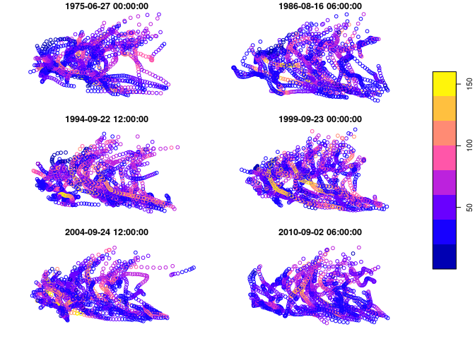
sftime has a simple plotting method. This will plot the spatial features and color them according to the values of a specified variable. The time values are assigned to intervals and for each interval, one panel is plotted with the panel title indicating the start time of the respective time interval. Here, we plot the storm records colored by their maximum sustained wind speed in knots:

plot(storms_sftime, y = "wind", key.pos = 4)

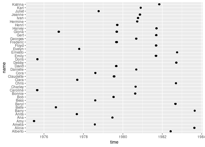
For other plots or more elaborated plots, we recommend using ggplot2 or tmap. For example, to plot when different storms (identified by their names) occurred, we can do:

library(ggplot2)

storms_sftime %>%
  dplyr::slice(1:1000) %>% # select only first 1000 records to keep things compact
  ggplot(aes (y = name, x = time)) +
  geom_point()

We’ll show a tmap plotting example in the next example.

Another motivating example: earthquake events

To illustrate sftime with another example, we’ll use data on earthquakes from the geostats package.

library(geostats)

# convert `earthquakes` data into an sftime object
earthquakes_sftime <- 
  earthquakes %>%
  dplyr::mutate(
    time = 
      paste(paste(year, month, day, sep = "-"), paste(hour, minute, second, sep = ":")) %>%
      as.POSIXct(format = "%Y-%m-%d %H:%M:%OS")
  ) %>%
  st_as_sftime(coords = c("lon", "lat"), time_column_name = "time", crs = 4326)

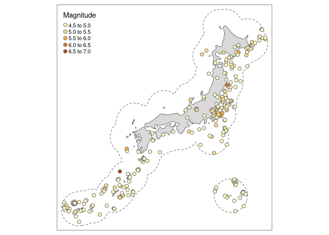
We want to filter the data for all earthquakes happening in Japan (including 200 km buffer) since 2020-01-01 and create a plot for this using tmap:

# get a polygon for Japan for filtering 
sf_japan <- 
  rnaturalearth::ne_countries(returnclass = "sf", scale = 'medium') %>% 
  dplyr::filter(name == "Japan") %>%
  st_transform(crs = 2451)

sf_japan_buffer <- 
  sf_japan %>%
  st_buffer(dist = 200 * 1000)

# filter the data
earthquakes_sftime_japan <- 
  earthquakes_sftime %>%
  st_transform(crs = 2451) %>%
  filter(time >= as.POSIXct("2020-01-01 00:00:00")) %>%
  st_filter(sf_japan_buffer, .predicate = st_within)

# plot with tmap
library(tmap)

tm_shape(sf_japan_buffer) + 
  tm_borders(lty = 2) +
  tm_shape(sf_japan) + 
  tm_polygons() +
  tm_shape(earthquakes_sftime_japan) +
  tm_bubbles(col = "mag", scale = 0.5, title.col = "Magnitude")

The `sftime` class

Object structure

The structure of sftime objects is simple when one already knows sf objects. sftime has an attribute time_column which defines one column of an sf object as active time column.

attributes(head(storms_sftime)) # head() to avoid too long output
#> $names
#>  [1] "name"        "year"        "status"      "category"    "wind"       
#>  [6] "pressure"    "ts_diameter" "hu_diameter" "geometry"    "time"       
#> 
#> $row.names
#> [1] 1 2 3 4 5 6
#> 
#> $sf_column
#> [1] "geometry"
#> 
#> $agr
#>        name        year      status    category        wind    pressure 
#>        <NA>        <NA>        <NA>        <NA>        <NA>        <NA> 
#> ts_diameter hu_diameter        time 
#>        <NA>        <NA>        <NA> 
#> Levels: constant aggregate identity
#> 
#> $class
#> [1] "sftime"     "sf"         "tbl_df"     "tbl"        "data.frame"
#> 
#> $time_column
#> [1] "time"

Conversion from and to `sftime`

sftime objects can be created from and converted to the following classes:

From	To	Methods	Side effects	Examples
To `sftime`
`sf` (package: `sf`)	`sftime`	`st_as_sftime()`, `st_sftime()`, `st_set_time()`		See this blogpost.
`stars` (package: `stars`)	`sftime`	`st_as_sftime()`		`st_as_sftime(stars::st_as_stars(earthquakes_sftime), time_column_name = "time")`
`sftime`	`sftime`	`st_as_sftime()`		`st_as_sftime(earthquakes_sftime)`
`data.frame` (package: `base`)	`sftime`	`st_as_sftime()`, `st_sftime()`		`st_as_sftime(as.data.frame(earthquakes_sftime), time_column_name = "time")`; `st_sftime(as.data.frame(earthquakes_sftime), time_column_name = "time")`
`tbl_df` (package: `tibble`)	`sftime`	`st_as_sftime()`, `st_sftime()`		`st_as_sftime(tibble::as_tibble(earthquakes_sftime), time_column_name = "time")`; `st_sftime(tibble::as_tibble(earthquakes_sftime), time_column_name = "time")`
`STI` (package: `spacetime`)	`sftime`	`st_as_sftime()`		See `?st_as_sftime`
`STIDF` (package: `spacetime`)	`sftime`	`st_as_sftime()`		See `?st_as_sftime`
`Track` (package: `trajectories`)	`sftime`	`st_as_sftime()`		See `?st_as_sftime`
`Tracks` (package: `trajectories`)	`sftime`	`st_as_sftime()`	Adds a column `track_name`.	See `?st_as_sftime`
`TracksCollection` (package: `trajectories`)	`sftime`	`st_as_sftime()`	Adds columns `track_name` and `tracks_name`.	See `?st_as_sftime`
From `sftime`
`sftime`	`data.frame` (package: `base`)	`as.data.frame()`		`as.data.frame(earthquakes_sftime)`
`sftime`	`tibble` (package: `tibble`)	`tibble::as_tibble()`		`tibble::as_tibble(earthquakes_sftime)`
`sftime`	`stars` (package: `stars`)	`stars::st_as_stars()`		`stars::st_as_stars(earthquakes_sftime)`
`sftime`	`sf` (package: `sf`)	`st_drop_time()`	drops active time column	`st_drop_time(earthquakes_sftime)`

Available methods

Currently, the following methods are available for sftime objects:

methods(class = "sftime")
#>  [1] [                 [[<-              $<-               anti_join        
#>  [5] arrange           cbind             distinct          filter           
#>  [9] full_join         group_by          inner_join        left_join        
#> [13] mutate            plot              print             rbind            
#> [17] rename            right_join        rowwise           sample_frac      
#> [21] sample_n          select            semi_join         slice            
#> [25] st_as_sftime      st_cast           st_crop           st_difference    
#> [29] st_drop_geometry  st_filter         st_intersection   st_join          
#> [33] st_sym_difference st_time           st_time<-         st_union         
#> [37] summarise         summarize         transform         transmute        
#> [41] ungroup          
#> see '?methods' for accessing help and source code

Outlook

`gstat` and `spcopula` integration

In the upcoming months, sftime will be integrated with gstat and spcopula to support spatiotemporal statistics (Kriging, spatiotemporal random fields) using sftime objects as input.

For example, irregular spatiotemporal data from weather stations (e.g. daily temperature records) can be spatiotemporally interpolated to compute a raster time series of temperature values for a certain area.

The general idea is that in these cases, an sftime object is the input for a spatiotemporal interpolation model, and a stars object is the output.

`sftime`: future developments

Also in the upcoming months, we will further develop the sftime package by adding still missing methods applicable to sf objects and conversion from sftrack and sftraj objects from the sftrack) package.

Any contributions here, including issues and pull requests are welcome.

Acknowledgment

This project gratefully acknowledges financial support from the

Which gap does the sftime package fill?