Processing satellite image collections in R with the gdalcubes package

The problem
Introduction and overview of gdalcubes
Installation
Demo dataset
Creating image collections
Creating and processing data cubes
Chaining data cube operations
User-defined functions
Interfacing with stars
Future work

The problem

Scientists working with collections and time series of satellite imagery quickly run into some of the following problems:

Images from different areas of the world have different spatial reference systems (e.g., UTM zones).
The pixel size of a single image sometimes differs among its spectral bands / variables.
Spatially adjacent image tiles often overlap.
Time series of images are often irregular when the area of interest covers spatial areas larger than the extent of a single image.
Images from different data products or different satellites are distributed in diverse data formats and structures.

GDAL and the rgdal R package can solve most of these difficulties by reading all relevant data formats and implementing image warping to reproject, rescale, resample, and crop images. However, GDAL does not know about image time series and hence there is a lot of manual work needed before data scientists can actually work with these data. Instead of collections of images, data users in many cases desire a regular data structure such as a four-dimensional raster data cube with dimensions x, y, time, and band.

In R, there is currently no implementation to build regular data cubes from image collections. The stars package provides a generic implementation for processing raster and vector data cubes with an arbitrary number of dimensions, but assumes that the data are already organized as an array.

Introduction and overview of gdalcubes

This blog post introduces the gdalcubes R package, aiming at making the work with collections and time series of satellite imagery easier and more interactive.

The core features of the package are:

build regular dense data cubes from large satellite image collections based on a user-defined data cube view (spatiotemporal extent, resolution, and map projection of the cube)
apply and chaining operations on data cubes
allow for the execution of user-defined functions on data cubes
export data cubes as netCDF files, making it easy to process further, e.g., with stars or raster.

Technically, the R package is a relatively lightweight wrapper around the gdalcubes C++ library. The library strongly builds on GDAL, netCDF, and SQLite (the full list of C++ libraries used by gdalcubes is found here).

This blog post focuses on how to use the R package gdalcubes, more details about the underlying ideas can be found in our recent open access paper in the datacube special issue of the DATA journal.

Installation

The package can be installed directly from CRAN:

install.packages("gdalcubes")

Some features and functions used in this blog post are still in the development version (which will be submitted to CRAN as version 0.2.0), which currently needs a source install:

# install.packages("remotes")
remotes::install_git("https://github.com/appelmar/gdalcubes_R", ref="dev", args="--recursive")

If this fails with error messages like “no rule to make target …”, please read here.

Demo dataset

We use a collection of 180 Landsat 8 surface reflectance images, covering a small part of the Brazilian Amazon forest. If you would like to work with the dataset on your own (and maybe reproduce some parts of this blog post), you have two options:

Option A: Download the dataset with full resolution (30 meter pixel size) here (67 gigabytes compressed; 190 gigabytes unzipped)

Option B: Download a downsampled version of the dataset that contains all images at a coarse spatial resolution (300 meter pixel size) here (740 megabytes compressed; 2 gigabytes unzipped)

Except for the spatial resolution of the images, the datasets are identical, meaning that all code samples work for both options but result images may look blurred when using option B. Here is the code to download and unzip the dataset to your current working directory (which might take some time):

# Option A
#download.file("https://uni-muenster.sciebo.de/s/SmiqWcCCeFSwfuY/download", destfile = "L8_Amazon.zip")

# Option B
if (!file.exists("L8_Amazon.zip")) {
  download.file("https://uni-muenster.sciebo.de/s/e5yUZmYGX0bo4u9/download", destfile = "L8_Amazon.zip")

  unzip("L8_Amazon.zip", exdir = "L8_Amazon")
}

Creating image collections

After extraction of the zip archive, we get one directory per image, where each image contains 10 GeoTIFF files representing the spectral bands and additional per-pixel quality information. As a first step, we must scan all available images once, extract some metadata (e.g. acquisition date/time and spatial extents of images and how the files relate to bands), and store this information in a simple image collection index file. This file does not store any pixel values but only metadata and references to where images can be found.

First, we simply need to find available GeoTIFF files in all subdirectories of our demo dataset:

files = list.files("L8_Amazon", recursive = TRUE, full.names = TRUE, pattern = ".tif")
length(files)

## [1] 1800

head(files)

## [1] "L8_Amazon/LC082260632014071901T1-SC20190715045926/LC08_L1TP_226063_20140719_20170421_01_T1_pixel_qa.tif"  
## [2] "L8_Amazon/LC082260632014071901T1-SC20190715045926/LC08_L1TP_226063_20140719_20170421_01_T1_radsat_qa.tif" 
## [3] "L8_Amazon/LC082260632014071901T1-SC20190715045926/LC08_L1TP_226063_20140719_20170421_01_T1_sr_aerosol.tif"
## [4] "L8_Amazon/LC082260632014071901T1-SC20190715045926/LC08_L1TP_226063_20140719_20170421_01_T1_sr_band1.tif"  
## [5] "L8_Amazon/LC082260632014071901T1-SC20190715045926/LC08_L1TP_226063_20140719_20170421_01_T1_sr_band2.tif"  
## [6] "L8_Amazon/LC082260632014071901T1-SC20190715045926/LC08_L1TP_226063_20140719_20170421_01_T1_sr_band3.tif"

To understand the structure of particular data products, the package comes with a set of predefined rules (called collection formats) that define how required metadata can be derived from the data. These include formats for some Sentinel-2, MODIS, and Landsat products. We can list all available formats with:

library(gdalcubes)

## Loading required package: Rcpp

## Loading required package: RcppProgress

## Loading required package: jsonlite

## Loading required package: ncdf4

## Using gdalcubes library version 0.1.9999

collection_formats()

##   CHIRPS_v2_0_daily_p05_tif | Image collection format for CHIRPS v 2.0
##                             | daily global precipitation dataset (0.05
##                             | degrees resolution) from GeoTIFFs, expects
##                             | list of .tif or .tif.gz files as input.
##                             | [TAGS: CHIRPS, precipitation]
## CHIRPS_v2_0_monthly_p05_tif | Image collection format for CHIRPS v 2.0
##                             | monthly global precipitation dataset (0.05
##                             | degrees resolution) from GeoTIFFs, expects
##                             | list of .tif or .tif.gz files as input.
##                             | [TAGS: CHIRPS, precipitation]
##                     L8_L1TP | Collection format for Landsat 8 Level 1 TP
##                             | product [TAGS: Landsat, USGS, Level 1, NASA]
##                       L8_SR | Collection format for Landsat 8 surface
##                             | reflectance product [TAGS: Landsat, USGS,
##                             | Level 2, NASA, surface reflectance]
##                     MxD10A2 | Collection format for selected bands from
##                             | the MODIS MxD10A2 (Aqua and Terra) v006 Snow
##                             | Cover product [TAGS: MODIS, Snow Cover]
##                     MxD11A1 | Collection format for selected bands from
##                             | the MODIS MxD11A2 (Aqua and Terra) v006 Land
##                             | Surface Temperature product [TAGS: MODIS,
##                             | LST]
##                     MxD11A2 | Collection format for selected bands from
##                             | the MODIS MxD11A2 (Aqua and Terra) v006 Land
##                             | Surface Temperature product [TAGS: MODIS,
##                             | LST]
##                     MxD13A3 | Collection format for selected bands from
##                             | the MODIS MxD13A3 (Aqua and Terra) product
##                             | [TAGS: MODIS, VI, NDVI, EVI]
##               Sentinel2_L1C | Image collection format for Sentinel 2 Level
##                             | 1C data as downloaded from the Copernicus
##                             | Open Access Hub, expects a list of file
##                             | paths as input. The format works on original
##                             | ZIP compressed as well as uncompressed
##                             | imagery. [TAGS: Sentinel, Copernicus, ESA,
##                             | TOA]
##           Sentinel2_L1C_AWS | Image collection format for Sentinel 2 Level
##                             | 1C data in AWS [TAGS: Sentinel, Copernicus,
##                             | ESA, TOA]
##               Sentinel2_L2A | Image collection format for Sentinel 2 Level
##                             | 2A data as downloaded from the Copernicus
##                             | Open Access Hub, expects a list of file
##                             | paths as input. The format should work on
##                             | original ZIP compressed as well as
##                             | uncompressed imagery. [TAGS: Sentinel,
##                             | Copernicus, ESA, BOA, Surface Reflectance]

The “L8_SR” format is what we need for our demo dataset. Next, we must tell gdalcubes to scan the files and build an image collection. Below, we create an image collection from the set of GeoTIFF files, using the “L8_SR” collection format and store the resulting image collection under “L8.db”.

L8.col = create_image_collection(files, "L8_SR", "L8.db")
L8.col

## A GDAL image collection object, referencing 180 images with 17  bands
## Images:
##                                       name      left       top    bottom
## 1 LC08_L1TP_226063_20140719_20170421_01_T1 -54.15776 -3.289862 -5.392073
## 2 LC08_L1TP_226063_20140820_20170420_01_T1 -54.16858 -3.289828 -5.392054
## 3 LC08_L1GT_226063_20160114_20170405_01_T2 -54.16317 -3.289845 -5.392064
## 4 LC08_L1TP_226063_20160724_20170322_01_T1 -54.16317 -3.289845 -5.392064
## 5 LC08_L1TP_226063_20170609_20170616_01_T1 -54.17399 -3.289810 -5.392044
## 6 LC08_L1TP_226063_20170711_20170726_01_T1 -54.15506 -3.289870 -5.392083
##       right            datetime
## 1 -52.10338 2014-07-19T00:00:00
## 2 -52.11418 2014-08-20T00:00:00
## 3 -52.10878 2016-01-14T00:00:00
## 4 -52.10878 2016-07-24T00:00:00
## 5 -52.11958 2017-06-09T00:00:00
## 6 -52.09798 2017-07-11T00:00:00
##                                                  srs
## 1 +proj=utm +zone=22 +datum=WGS84 +units=m +no_defs 
## 2 +proj=utm +zone=22 +datum=WGS84 +units=m +no_defs 
## 3 +proj=utm +zone=22 +datum=WGS84 +units=m +no_defs 
## 4 +proj=utm +zone=22 +datum=WGS84 +units=m +no_defs 
## 5 +proj=utm +zone=22 +datum=WGS84 +units=m +no_defs 
## 6 +proj=utm +zone=22 +datum=WGS84 +units=m +no_defs 
## [ omitted 174 images ] 
## 
## Bands:
##         name offset scale unit       nodata image_count
## 1    AEROSOL      0     1                           180
## 2        B01      0     1      -9999.000000         180
## 3        B02      0     1      -9999.000000         180
## 4        B03      0     1      -9999.000000         180
## 5        B04      0     1      -9999.000000         180
## 6        B05      0     1      -9999.000000         180
## 7        B06      0     1      -9999.000000         180
## 8        B07      0     1      -9999.000000         180
## 9        EVI      0     1      -9999.000000           0
## 10     MSAVI      0     1      -9999.000000           0
## 11       NBR      0     1      -9999.000000           0
## 12      NBR2      0     1      -9999.000000           0
## 13      NDMI      0     1      -9999.000000           0
## 14      NDVI      0     1      -9999.000000           0
## 15  PIXEL_QA      0     1                           180
## 16 RADSAT_QA      0     1                           180
## 17      SAVI      0     1      -9999.000000           0

Internally, the output file is a simple SQLite database. Please notice that our collection does not contain data for all possible bands (see image_count column). Depending on particular data download requests, Landsat 8 surface reflectance data may come e.g. with some post-processed bands (like vegetation indexes) that can be used if available.

Creating and processing data cubes

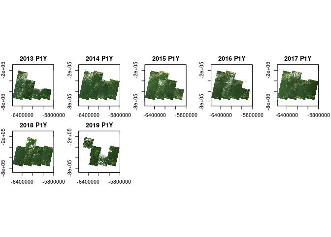
To create a raster data cube, we need (i) an image collection and (ii) a data cube view, defining how we look at the data, i.e., at which spatiotemporal resolution, window, and spatial reference system. For a quick look at the data, we define a cube view with 1km x 1km pixel size, yearly temporal resolution, covering the full spatiotemporal extent of the image collection, and using the web mercator spatial reference system.

v.overview = cube_view(extent=L8.col, dt="P1Y", dx=1000, dy=1000, srs="EPSG:3857", 
                       aggregation = "median", resampling = "bilinear")
raster_cube(L8.col, v.overview)

## A GDAL data cube proxy object
## Dimensions:
##   name        low       high size chunk_size
## 1    t     2013.0     2019.0    7         16
## 2    y  -764014.4  -205014.4  559        256
## 3    x -6582280.1 -5799280.1  783        256
## 
## Bands:
##         name    type offset scale nodata unit
## 1    AEROSOL float64      0     1    NaN     
## 2        B01 float64      0     1    NaN     
## 3        B02 float64      0     1    NaN     
## 4        B03 float64      0     1    NaN     
## 5        B04 float64      0     1    NaN     
## 6        B05 float64      0     1    NaN     
## 7        B06 float64      0     1    NaN     
## 8        B07 float64      0     1    NaN     
## 9        EVI float64      0     1    NaN     
## 10     MSAVI float64      0     1    NaN     
## 11       NBR float64      0     1    NaN     
## 12      NBR2 float64      0     1    NaN     
## 13      NDMI float64      0     1    NaN     
## 14      NDVI float64      0     1    NaN     
## 15  PIXEL_QA float64      0     1    NaN     
## 16 RADSAT_QA float64      0     1    NaN     
## 17      SAVI float64      0     1    NaN

As specified in our data cube view, the time dimension of the resulting data cube only has 7 values, representing years from 2013 to 2019. The aggregation parameter in the data cube view defines how values from multiple images in the same year shall be combined. In contrast, the selected resampling algorithm is applied when reprojecting and rescaling individual images.

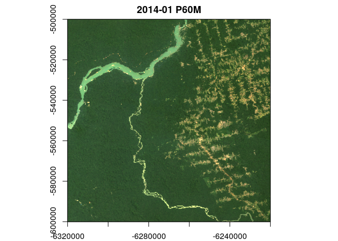
If we are interested in a smaller area at higher temporal resolution, we simply need to define a data cube view with different parameters, including a specific spatiotemporal extent by passing a list as extent argument to cube_view. Below, we define a data cube view for a 100km x 100km area with 50m pixel size at monthly temporal resolution.

v.subarea = cube_view(extent=list(left=-6320000, right=-6220000, bottom=-600000, top=-500000, 
                      t0="2014-01-01", t1="2018-12-31"), dt="P1M", dx=50, dy=50, srs="EPSG:3857", 
                      aggregation = "median", resampling = "bilinear")

raster_cube(L8.col, v.subarea)

## A GDAL data cube proxy object
## Dimensions:
##   name      low     high size chunk_size
## 1    t   201401   201812   60         16
## 2    y  -600000  -500000 2000        256
## 3    x -6320000 -6220000 2000        256
## 
## Bands:
##         name    type offset scale nodata unit
## 1    AEROSOL float64      0     1    NaN     
## 2        B01 float64      0     1    NaN     
## 3        B02 float64      0     1    NaN     
## 4        B03 float64      0     1    NaN     
## 5        B04 float64      0     1    NaN     
## 6        B05 float64      0     1    NaN     
## 7        B06 float64      0     1    NaN     
## 8        B07 float64      0     1    NaN     
## 9        EVI float64      0     1    NaN     
## 10     MSAVI float64      0     1    NaN     
## 11       NBR float64      0     1    NaN     
## 12      NBR2 float64      0     1    NaN     
## 13      NDMI float64      0     1    NaN     
## 14      NDVI float64      0     1    NaN     
## 15  PIXEL_QA float64      0     1    NaN     
## 16 RADSAT_QA float64      0     1    NaN     
## 17      SAVI float64      0     1    NaN

The raster_cube function always returns a proxy object, meaning that neither any expensive computations nor any data reads from disk are started. Instead, gdalcubes delays the execution until the data is really needed when users call plot(), or write_ncdf(). However, the result of our call to raster_cube can be passed to data cube operators. For example, the code below drops all bands except the visible RGB bands and, again, returns a proxy object.

L8.cube.rgb = select_bands(raster_cube(L8.col, v.overview), c("B02","B03","B04")) 
L8.cube.rgb 

## A GDAL data cube proxy object
## Dimensions:
##   name        low       high size chunk_size
## 1    t     2013.0     2019.0    7         16
## 2    y  -764014.4  -205014.4  559        256
## 3    x -6582280.1 -5799280.1  783        256
## 
## Bands:
##   name    type offset scale nodata unit
## 1  B02 float64      0     1    NaN     
## 2  B03 float64      0     1    NaN     
## 3  B04 float64      0     1    NaN

Calling plot() will eventually start computationn, and hence might take some time:

system.time(plot(L8.cube.rgb, rgb=3:1, zlim=c(0,1200)))

##    user  system elapsed 
##  16.367   0.605  17.131

Chaining data cube operations

For the remaining examples, we use multiple threads to process data cubes by setting:

gdalcubes_options(threads=4)

We can chain many of the provided data cube operators (e.g., using the pipe %>%). The following code will derive the median values of the RGB bands over time, producing a single RGB overview image for our selected subarea.

suppressPackageStartupMessages(library(magrittr)) # use the pipe
raster_cube(L8.col, v.subarea) %>%
  select_bands(c("B02","B03","B04")) %>%
  reduce_time("median(B02)", "median(B03)", "median(B04)") %>%
  plot(rgb=3:1, zlim=c(0,1200))

Implemented data cube operators include:

apply_pixel apply one or more arithmetic expressions on individual data cube pixels, e.g., to derive vegetation indexes.
reduce_time apply on or more reducers over pixel time series.
reduce_time apply on or more reducers over spatial slices.
select_bands subset available bands.
window_time apply an aggregation function or convolution kernel over moving time series windows.
join_bands combines the bands of two indentically shaped data cubes.
filter_pixel filter pixels by a logical expression on band values, e.g., select all pixels with NDVI larger than 0.
write_ncdf export a data cube as a netCDF file.

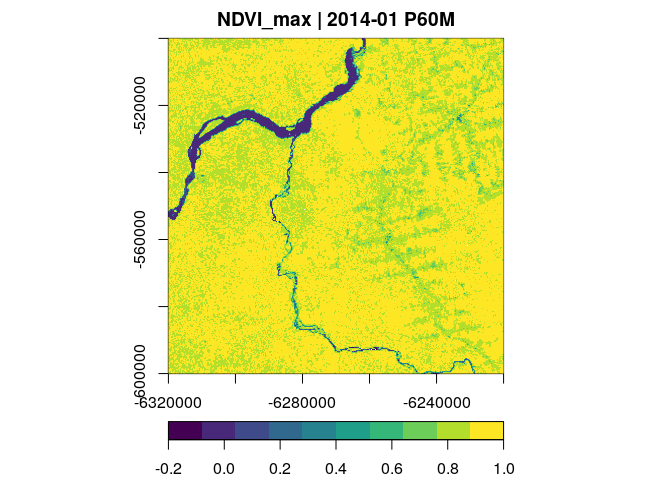
In a second example, we compute the normalied difference vegetation index (NDVI) with apply_pixel and derive its maximum values over time:

suppressPackageStartupMessages(library(viridis)) # use colors from viridis package

raster_cube(L8.col, v.subarea) %>%
  select_bands(c("B04","B05")) %>%
  apply_pixel(c("(B05-B04)/(B05+B04)"), names="NDVI") %>%
  reduce_time("max(NDVI)") %>%
  plot(zlim=c(-0.2,1), col=viridis, key.pos=1)

User-defined functions

Previous examples used character expressions to define reducer and arithmetic functions. Operations like apply_pixel and filter_pixel take character arguments to define the expressions. The reason for this is that expressions are translated to C++ functions and all computations then are purely C++. However, to give users more flexibility and allow the definition of user-defined functions, reduce_time and apply_pixel also allow to pass arbitrary R functions as an argument. 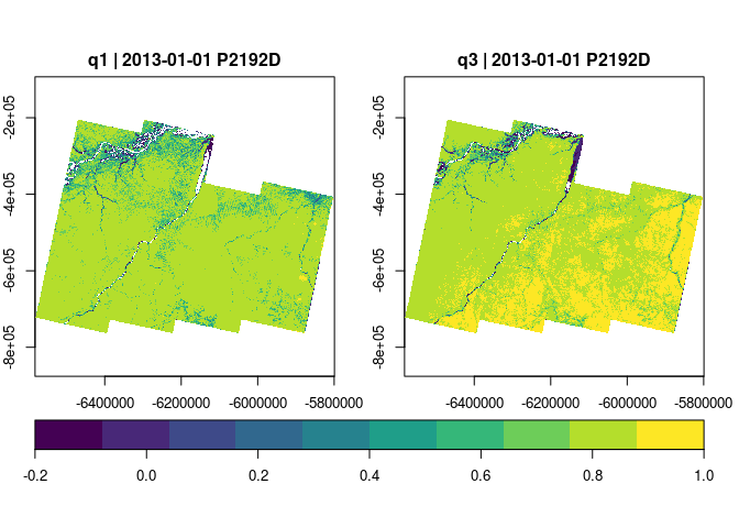In the example below, we derive the 0.25, and 0.75 quantiles over NDVI time series. There is of course no limitation what the provided reducer function does and it is thus possible to use functions from other packages.

v.16d = cube_view(view=v.overview, dt="P16D")
raster_cube(L8.col, v.16d) %>%
  select_bands(c("B04", "B05")) %>%
  apply_pixel(c("(B05-B04)/(B05+B04)"), names="NDVI") %>%
  reduce_time(names = c("q1","q3"), FUN = function(x) {
    quantile(x["NDVI",], probs = c(0.25, 0.75), na.rm = TRUE)
  }) %>%
  plot(col=viridis, zlim=c(-0.2,1), key.pos=1)

However, there are some things, users need to keep in mind when working with user-defined functions:

Users should provide names of the output bands and make sure that the function always return the same number of elements.
When executed, the function runs in a new R session, meaning that it cannot access variables in the current worskspace and packages must be loaded within the function if needed.
Ideally, users should carefully check for errors. A frequent cause for errors is the presence of NA values, which are abundant in raster data cubes from irregular image collections.
In the current version, only apply_pixel and reduce_time allow for passing user-defined functions.

Interfacing with stars

The stars package is much more generic and supports higher dimensional arrays and hence supports e.g. data from climate model output. It also does not assume data to be orthorectified, i.e. it works also with curvilinear grids and hence supports data as from Sentinel-5P. In contrast, gdalcubes concentrates on multispectral image time series (4d) only.

gdalcubes currently comes with a simple as_stars() function, writing a data cube as a (temporary) netCDF file, which is then opened by read_stars. The stars object holds bands as attributes. If needed (e.g. for ggplot below), st_redimension converts attributes to a new dimension.

suppressPackageStartupMessages(library(ggplot2))
suppressPackageStartupMessages(library(dplyr))
suppressPackageStartupMessages(library(stars))

x = raster_cube(L8.col, v.overview) %>%
  select_bands(c("B02","B03","B04")) %>%
  as_stars()
x

## stars object with 3 dimensions and 3 attributes
## attribute(s), summary of first 1e+05 cells:
##       B02              B03              B04         
##  Min.   : 123.8   Min.   : 174.1   Min.   :  112.1  
##  1st Qu.: 209.9   1st Qu.: 397.3   1st Qu.:  247.2  
##  Median : 295.0   Median : 497.9   Median :  380.3  
##  Mean   : 457.6   Mean   : 653.0   Mean   :  563.5  
##  3rd Qu.: 476.7   3rd Qu.: 686.5   3rd Qu.:  662.6  
##  Max.   :9419.0   Max.   :9780.7   Max.   :10066.2  
##  NA's   :79497    NA's   :79497    NA's   :79497    
## dimension(s):
##      from  to   offset delta                       refsys point
## x       1 783 -6582280  1000 +proj=merc +a=6378137 +b=... FALSE
## y       1 559  -205014 -1000 +proj=merc +a=6378137 +b=... FALSE
## time    1   7       NA    NA                      POSIXct FALSE
##                         values    
## x                         NULL [x]
## y                         NULL [y]
## time 2013-01-01,...,2019-01-01

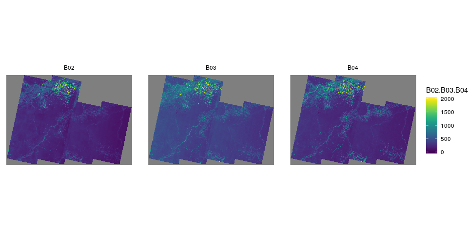
ggplot() + 
  geom_stars(data = slice(st_redimension(x), "time", 5)) + 
  facet_wrap(~new_dim) + 
  theme_void() +
  coord_fixed() +
  scale_fill_viridis(limits=c(0, 2000)) 

Future work

There are many things, which we didn’t cover in this blog post like applying masks during the construction of data cubes. More importantly, a question we are very much interested in at the moment is how far we can go with gdalcubes and stars in cloud computing envrionments, where huge image collections such as the full Sentinel-2 archive are already stored. This will be the topic of another blog post.

We also have a lot of ideas for future developments but no real schedule. If you would like to contribute, get involved, or if you have further ideas, please get in touch! Development and discussion takes place on GitHub (R package on GitHub, C++ library on GitHub ).