sf 0.6-0 news
- Ring directions
- Higher-order geometry differences
- Spherical geometry
- Hausdorff and Frechet distance
- snap!
- join to largest matching feature
- polygon geometries have zero length
- printing coordinates now honors
digitssetting
Version 0.6-0 of the sf package (an R package for handling vector geometries in R) has been released to CRAN. It contains several innovations, summarized in the NEWS file. This blog post will illustrate some of these further.
Ring directions
Consider the following two polygons:
library(sf)

## Loading required package: methods

## Linking to GEOS 3.5.1, GDAL 2.1.2, proj.4 4.9.3

p1 = rbind(c(0,0), c(1,0), c(1,1), c(0,1), c(0,0))
p2 = 0.5 * p1 + 0.25
(pol1 = st_polygon(list(p1, p2)))

## POLYGON ((0 0, 1 0, 1 1, 0 1, 0 0), (0.25 0.25, 0.75 0.25, 0.75 0.75, 0.25 0.75, 0.25 0.25))

(pol2 = st_polygon(list(p1, p2[5:1,])))

## POLYGON ((0 0, 1 0, 1 1, 0 1, 0 0), (0.25 0.25, 0.25 0.75, 0.75 0.75, 0.75 0.25, 0.25 0.25))

opar = par(mfrow = c(1, 2), mar = rep(0, 4))
plot(pol1, col = grey(.8), rule = "winding")
plot(pol2, col = grey(.8), rule = "winding")
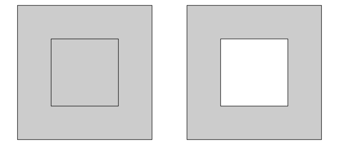
Although the simple feature standard describes that all secondary rings
indicate holes, it also specifies that outer rings should be counter
clockwise and inner rings (holes) clockwise. It doesn’t specify that
polygons for which the hole has the same ring direction as the outer
ring are invalid - and they aren’t. But how should software deal with
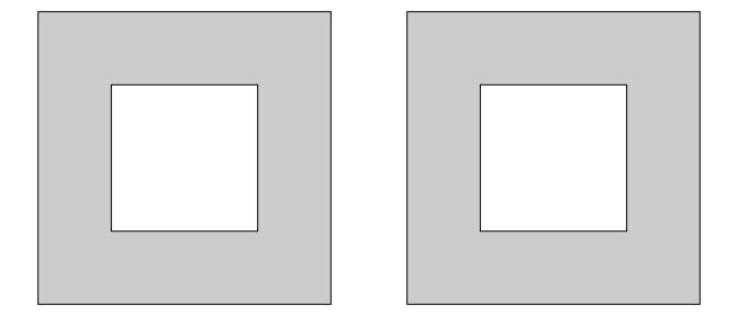
them? In prior sf versions, plot (and ggplot) would take the
winding rule, requiring holes to have the opposite direction as outer
rings. This has been changed into evenodd as default, which plots both
cases with holes:
library(sf)
p1 = rbind(c(0,0), c(1,0), c(1,1), c(0,1), c(0,0))
p2 = 0.5 * p1 + 0.25
(pol1 = st_polygon(list(p1, p2)))

## POLYGON ((0 0, 1 0, 1 1, 0 1, 0 0), (0.25 0.25, 0.75 0.25, 0.75 0.75, 0.25 0.75, 0.25 0.25))

(pol2 = st_polygon(list(p1, p2[5:1,])))

## POLYGON ((0 0, 1 0, 1 1, 0 1, 0 0), (0.25 0.25, 0.25 0.75, 0.75 0.75, 0.75 0.25, 0.25 0.25))

opar = par(mfrow = c(1, 2), mar = rep(0, 4))
plot(pol1, col = grey(.8)) # rule = "evenodd"
plot(pol2, col = grey(.8)) # rule = "evenodd"
In addition, st_sfc and st_read gained a parameter check_ring_dir,
by default FALSE, which when TRUE will check every ring and revert
them to counter clockwise for outer, and clockwise for inner (hole)
rings. By default this is FALSE because it is an expensive operation
for large datasets.
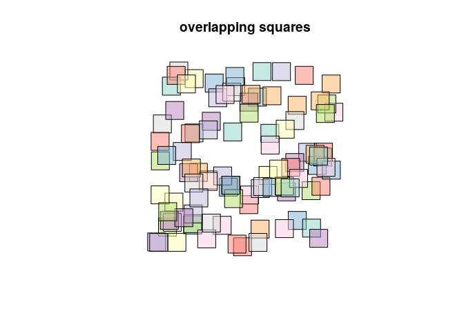
Higher-order geometry differences
This was reported here;
two nice graphs are available from ?st_difference
set.seed(131)
m = rbind(c(0,0), c(1,0), c(1,1), c(0,1), c(0,0))
p = st_polygon(list(m))
n = 100
l = vector("list", n)
for (i in 1:n)
l[[i]] = p + 10 * runif(2)
s = st_sfc(l)
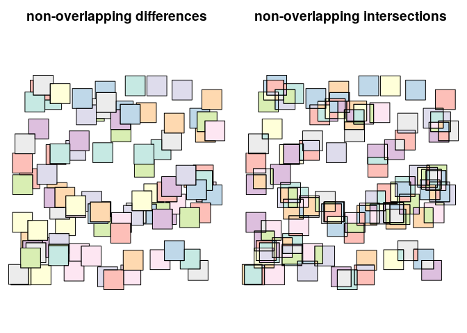
d = st_difference(s) # sequential differences: s1, s2-s1, s3-s2-s1, ...
i = st_intersection(s) # all intersections
plot(s, col = sf.colors(categorical = TRUE, alpha = .5))
title("overlapping squares")
par(mfrow = c(1, 2), mar = c(0,0,2.4,0))
plot(d, col = sf.colors(categorical = TRUE, alpha = .5))
title("non-overlapping differences")
plot(i, col = sf.colors(categorical = TRUE, alpha = .5))
title("non-overlapping intersections")
Spherical geometry
All geometric operations (area, length, intersects, intersection, union etc) provided by the GEOS library assume two-dimensional coordinates. If your data have geographic (longitude-latitude) coordinates, this is may be quite OK when your area is small and close to the equator, otherwise it is not. One way out is to project the data using a suitable projection, the other is to use spherical geometry: algorithms that compute on the sphere (or, more precisely, on the spheroid. This has a number of advantages:
- it is easy, you have no-worries about which projection to choose
- it is always correct
however, it comes at some computational cost.
Spherical geometry functions were formerly taken from R package
geosphere; with the new sf they use package
lwgeom,
which interfaces liblwgeom, the library that is also used by PostGIS. (and the
development of which was funded by
palantir).
Liblwgeom functions st_make_valid, st_geohash, st_split, which were
formerly in sf have now been moved to lwgeom. Other functions in
lwgeom enable the following functions to work with geographic
coordinates: st_length, st_area st_distance,
st_is_within_distance, st_segmentize.
Where geosphere could only compute distances between points,
st_distance now computes distances between arbitrary simple feature
geometries. st_distance is clearly slower when computed on a spheroid
than when computed on the sphere. For point data, faster results are
obtained when we assume the Earth is a sphere:
n = 2000
df = data.frame(x = runif(n), y = runif(n))
pts = st_as_sf(df, coords = c("x", "y"))
system.time(x0 <- st_distance(pts))

##    user  system elapsed
##   3.456   0.008   3.479

st_crs(pts) = 4326 # spheroid
system.time(x1 <- st_distance(pts))

##    user  system elapsed
##   5.564   0.016   5.594

st_crs(pts) = "+proj=longlat +ellps=sphere" # sphere

## Warning: st_crs<- : replacing crs does not reproject data; use st_transform
## for that

system.time(x2 <- st_distance(pts))

##    user  system elapsed
##   1.220   0.024   1.246

system.time(x3 <- dist(as.matrix(df)))

##    user  system elapsed
##   0.012   0.000   0.010
Hausdorff and Frechet distance
For two-dimensional (flat) geometries, st_distance now has the option
of computing Hausdorff
distances, and (if
sf was linked to GEOS 3.7.0) Frechet
distances.
snap!
For two-dimensional (flat) geometries, st_snap is now available; we
refer to the PostGIS
documentation for examples what it does.
join to largest matching feature
This feature was reported and illustrated here:
sf::st_join with “largest=TRUE” now joins to the single largest intersecting feature: https://t.co/qqdLonBuKL #rspatial #rstats pic.twitter.com/6oVhlYdb5Z
— Edzer Pebesma (@edzerpebesma) December 3, 2017
polygon geometries have zero length
Function st_length now returns zero for non-linear geometries
including polygons. For length of polygon rings, st_cast to
MULTILINESTRING first.
printing coordinates now honors digits setting
Printing of geometries, as well as st_as_text now use the default
digits of R:
st_point(c(1/3, 1/6))

## POINT (0.3333333 0.1666667)

options(digits = 3)
st_point(c(1/3, 1/6))

## POINT (0.333 0.167)

st_as_text(st_point(c(1/3, 1/6)), digits = 16)

## [1] "POINT (0.3333333333333333 0.1666666666666667)"
Before sf 0.6, as.character was used, which used around 16 digits.