Spatiotemporal arrays for R - blog one
- Update
- Summary
- Introduction
- Reading a satellite image
- Affine grids
- Reading a raster time series: netcdf
- More complex arrays
- Raster layers and bricks
- Next steps
- Reactions
Update
Since this blog post, the stars API has changed; a version of this blog post that has been kept up-to-date with the software is found here, or available from the package as vignette("blog1").
Summary
This is the first blog on the
stars project, an R-Consortium
funded project for spatiotemporal tidy arrays with R. It shows how
stars combines bands and/or subdatasets of GDAL datasets (data cubes)
into R arrays with well-referenced space and time dimensions, how it
deals with affine (rotated) grids, and how it interfaces to packages
dplyr, sf and raster. An artificial example shows the creation of
an origin-destination matrix by travel mode and time.
Introduction
The goals of the stars project are
- to handle raster data in a way that integrates well with the sf project and with the tidyverse
- to handle array data (time series, or otherwise functional data) where time and space are among the dimensions
- to do this in a scalable way, i.e. deal with cases where data are too large to fit in memory or on disk
- to think about a migration path for the large and famous raster in the same directions
In its current stage stars and (as planned) does not have
- scalability to large data sets; everything is still in memory
- writing data back to disk
The package is loaded by
# devtools::install_github("r-spatial/stars")
library(stars)
## Loading required package: dplyr
##
## Attaching package: 'dplyr'
## The following objects are masked from 'package:stats':
##
##     filter, lag
## The following objects are masked from 'package:base':
##
##     intersect, setdiff, setequal, union
## Loading required package: magrittr
## Loading required package: sf
## Loading required package: methods
## Linking to GEOS 3.5.1, GDAL 2.1.2, proj.4 4.9.3
## Linking to GDAL 2.1.2
The stars package links natively to GDAL; all I/O is done through
direct calls to GDAL functions, without using sf or rgdal.
Spatiotemporal arrays are stored in objects of class stars, and
methods for class stars currently include:
methods(class = "stars")
##  [1] aperm         as.data.frame as.tbl_cube   c             coerce
##  [6] dim           filter        image         initialize    mutate
## [11] print         pull          select        show          slotsFromS3
## [16] st_as_sf      st_as_sfc     st_bbox       st_crs        st_dimensions
## see '?methods' for accessing help and source code
Note that everything in the stars api may still be subject to change
in the next few months.
Reading a satellite image
We can read a satellite image through GDAL, e.g. from a GeoTIFF file in the package:
tif = system.file("tif/L7_ETMs.tif", package = "stars")
x <- tif %>% st_stars
par(mar = rep(0,4))
image(x, col = grey((4:10)/10))
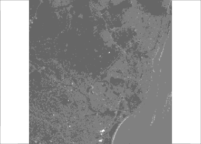
From the following output, we can see that the image is geographically
referenced, and that the object returned (x) has three dimensions:
x, y and band, and one attribute:
x
## stars object with 3 dimensions and 1 attribute
## attribute(s), of first 1e+05 cells:
##  /home/edzer/R/x86_64-pc-linux-gnu-library/3.4/stars/tif/L7_ETMs.tif
##  Min.   : 47.00
##  1st Qu.: 65.00
##  Median : 76.00
##  Mean   : 77.34
##  3rd Qu.: 87.00
##  Max.   :255.00
## dimension(s):
##      from  to  offset delta
## x       1 349  288776  28.5
## y       1 352 9120761 -28.5
## band    1   6      NA    NA
##                                                                                refsys
## x    +proj=utm +zone=25 +south +ellps=GRS80 +towgs84=0,0,0,0,0,0,0 +units=m +no_defs
## y    +proj=utm +zone=25 +south +ellps=GRS80 +towgs84=0,0,0,0,0,0,0 +units=m +no_defs
## band                                                                               NA
##      point values
## x    FALSE   NULL
## y    FALSE   NULL
## band    NA   NULL
Each dimension has a name; the meaning of the fields of a single dimension are:
| field | meaning |
|---|---|
| from | the origin index (1) |
| to | the final index (dim(x)[i]) |
| offset | the start value for this dimension |
| delta | the step size for this dimension |
| refsys | the reference system, or proj4string |
| point | logical; whether cells refer to points, or intervals |
| values | the sequence of values for this dimension (e.g., geometries) |
This means that for an index i (starting at \(i=1\)) along a certain dimension, the corresponding dimension value (coordinate, time) is \(\mbox{offset} + (i-1) \times \mbox{delta}\). This value then refers to the start (edge) of the cell or interval; in order to get the interval middle or cell centre, one needs to add half an offset.
Dimension band is a simple sequence from 1 to 6. Although bands refer
to colors, their wavelength (color) values are not available.
For this particular dataset (and most other raster datasets), we see
that offset for dimension y is negative: this means that consecutive
array values have decreasing \(y\) values: cells are ordered from top
to bottom, opposite the direction of the \(y\) axis.
st_stars reads all bands from a raster dataset, or a set of raster
datasets, into a single stars array structure. While doing so, raster
values (often UINT8 or UINT16) are converted to double (numeric) values,
and scaled back to their original values if needed.
The data structure stars resembles the tbl_cube found in dplyr; we
can convert to that by
as.tbl_cube(x)
## Source: local array [737,088 x 3]
## D: x [dbl, 349]
## D: y [dbl, 352]
## D: band [int, 6]
## M: /home/edzer/R/x86_64-pc-linux-gnu-library/3.4/stars/tif/L7_ETMs.tif [dbl]
In contrast to stars objects, tbl_cube objects
- do not explicitly handle regular dimensions (offset, delta)
- do not register reference systems (unless they are a single dimension property)
- do not cope with affine grids (see below)
- do not cope with dimensions represented by a list (e.g. simple features, see below)
- do not register whether attribute values (measurements) refer to point or interval values, on each dimension
Affine grids
The GDAL model can deal also with spatial rasters that are regular but not aligned with \(x\) and \(y\): affine grids. An example is given here:
par(cex.axis = .7) # font size axis tic labels
geomatrix = system.file("tif/geomatrix.tif", package = "stars")
geomatrix %>% st_stars %>% st_as_sf(as_points = FALSE) %>%
  plot(axes =TRUE, main = "geomatrix.tif", graticule = TRUE)
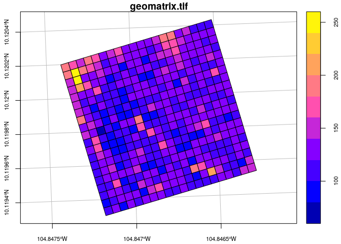
Looking at the dimensions
geomatrix %>% st_stars %>% st_dimensions
##   from to  offset delta                        geotransform
## x    1 20 1841002   1.5 1841000, 1.5, -5, 1144000, -5, -1.5
## y    1 20 1144003  -1.5 1841000, 1.5, -5, 1144000, -5, -1.5
##                                               refsys point values
## x +proj=utm +zone=11 +datum=WGS84 +units=m +no_defs   TRUE   NULL
## y +proj=utm +zone=11 +datum=WGS84 +units=m +no_defs   TRUE   NULL
further reveals that we now have a geotransform field shown in the
dimension table; this is only displayed when the affine parameters are
non-zero. The geotransform field has six parameters, \(gt_1,…,gt_6\)
that are used to transform internal raster coordinates (column pixel
\(i\) and row pixel \(j\)) to world coordinates (\(x\), \(y\)):
\[x = gt_1 + (i-1) gt_2 + (j-1) gt_3\]
\[y = gt_4 + (i-1) gt_5 + (j-1) gt_6\]
When \(gt_3\) and \(gt_5\) are zero, the \(x\) and \(y\) are parallel to \(i\) and \(j\), which makes it appear unrotated.
Reading a raster time series: netcdf
Another example is when we read raster time series model outputs in a NetCDF file, e.g. by
prec = st_stars("data/full_data_daily_2013.nc")
## p, sd, ek, s,
(Note that this 380 Mb file is not included; data are described here, and were downloaded from here).
We see that
prec
## stars object with 3 dimensions and 4 attributes
## attribute(s), of first 1e+05 cells:
##   p [(mm/day)]    sd [(mm/day)]       ek [%]       s [gauges per gridcell]
##  Min.   :  0.00   Min.   : 0.00   Min.   :  1.02   Min.   :-99999
##  1st Qu.:  0.00   1st Qu.: 0.00   1st Qu.: 15.38   1st Qu.:-99999
##  Median :  0.10   Median : 0.16   Median : 24.70   Median :-99999
##  Mean   :  1.71   Mean   : 1.74   Mean   : 29.72   Mean   :-65915
##  3rd Qu.:  0.97   3rd Qu.: 1.14   3rd Qu.: 40.20   3rd Qu.:     0
##  Max.   :133.53   Max.   :73.51   Max.   :100.00   Max.   :   101
##  NA's   :66000    NA's   :66000   NA's   :66000
## dimension(s):
##      from  to     offset  delta  refsys point values
## x       1 360       -180      1      NA    NA   NULL
## y       1 180         90     -1      NA    NA   NULL
## time    1 365 2013-01-01 1 days POSIXct    NA   NULL
For this dataset we can see that
- variables have units associated
- time is now a dimension, with proper units and time steps
- missing values for the fourth variable were not taken care off correctly
Reading datasets from multiple files
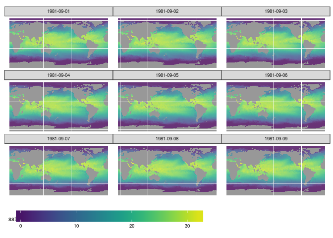
Model data are often spread across many files. An example of a 0.25 degree grid, global daily sea surface temperature product is found here; a subset of the 1981 data was downloaded from here.
We read the data by giving st_stars a vector with character names:
x = c(
"avhrr/avhrr-only-v2.19810901.nc",
"avhrr/avhrr-only-v2.19810902.nc",
"avhrr/avhrr-only-v2.19810903.nc",
"avhrr/avhrr-only-v2.19810904.nc",
"avhrr/avhrr-only-v2.19810905.nc",
"avhrr/avhrr-only-v2.19810906.nc",
"avhrr/avhrr-only-v2.19810907.nc",
"avhrr/avhrr-only-v2.19810908.nc",
"avhrr/avhrr-only-v2.19810909.nc"
)

(y = st_stars(x, quiet = TRUE))
## stars object with 4 dimensions and 4 attributes
## attribute(s), of first 1e+05 cells:
##  sst [degrees C] anom [degrees C] err [degrees C] ice [percentage]
##  Min.   :-1.80   Min.   :-4.69    Min.   :0.110   Min.   :0.010
##  1st Qu.:-1.19   1st Qu.:-0.06    1st Qu.:0.300   1st Qu.:0.730
##  Median :-1.05   Median : 0.52    Median :0.300   Median :0.830
##  Mean   :-0.32   Mean   : 0.23    Mean   :0.295   Mean   :0.766
##  3rd Qu.:-0.20   3rd Qu.: 0.71    3rd Qu.:0.300   3rd Qu.:0.870
##  Max.   : 9.36   Max.   : 3.70    Max.   :0.480   Max.   :1.000
##  NA's   :13360   NA's   :13360    NA's   :13360   NA's   :27377
## dimension(s):
##      from   to     offset  delta  refsys point values
## x       1 1440          0   0.25      NA    NA   NULL
## y       1  720         90  -0.25      NA    NA   NULL
## time    1    9 1981-09-01 1 days POSIXct    NA   NULL
## zlev    1    1   0 meters     NA      NA    NA   NULL
Next, we select sea surface temperature (sst), and drop the singular
zlev (depth) dimension using adrop:
library(abind)
z <- y %>% select(sst) %>% adrop
We can now graph the sea surface temperature (SST) using ggplot, which
needs data in a long table form, and without units:
df = as.data.frame(z)
df$sst = unclass(df$sst)
library(ggplot2)
library(viridis)
## Loading required package: viridisLite
library(ggthemes)
ggplot() +
  geom_tile(data=df, aes(x=x, y=y, fill=sst), alpha=0.8) +
  facet_wrap("time") +
  scale_fill_viridis() +
  coord_equal() +
  theme_map() +
  theme(legend.position="bottom") +
  theme(legend.key.width=unit(2, "cm"))
More complex arrays
Like tbl_cube, stars arrays have no limits to the number of
dimensions they handle. An example is the origin-destination (OD)
matrix, by time and travel mode.
OD: space x space x travel mode x time x time
We create a 5-dimensional matrix of traffic between regions, by day, by time of day, and by travel mode. Having day and time of day each as dimension is an advantage when we want to compute patters over the day, for a certain period.
nc = read_sf(system.file("gpkg/nc.gpkg", package="sf"))
to = from = st_geometry(nc) # 100 polygons: O and D regions
mode = c("car", "bike", "foot") # travel mode
day = 1:100 # arbitrary
library(units)
units(day) = make_unit("days since 2015-01-01")
hour = set_units(0:23, h) # hour of day
dims = st_dimensions(origin = from, destination = to, mode = mode, day = day, hour = hour)
(n = dim(dims))
##      origin destination        mode         day        hour
##         100         100           3         100          24
traffic = array(rpois(prod(n), 10), dim = n) # simulated traffic counts
(st = st_stars(list(traffic = traffic),  dimensions = dims))
## stars object with 5 dimensions and 1 attribute
## attribute(s), of first 1e+05 cells:
##     traffic
##  Min.   : 0
##  1st Qu.: 8
##  Median :10
##  Mean   :10
##  3rd Qu.:12
##  Max.   :25
## dimension(s):
##             from  to                    offset                     delta
## origin         1 100                        NA                        NA
## destination    1 100                        NA                        NA
## mode           1   3                        NA                        NA
## day            1 100 1 (days since 2015-01-01) 1 (days since 2015-01-01)
## hour           1  24                       0 h                       1 h
##                                          refsys point
## origin      +proj=longlat +datum=NAD27 +no_defs    NA
## destination +proj=longlat +datum=NAD27 +no_defs    NA
## mode                                         NA    NA
## day                                          NA    NA
## hour                                         NA    NA
##                                                                          values
## origin      MULTIPOLYGON (((-81.4727554..., ..., MULTIPOLYGON (((-78.6557159...
## destination MULTIPOLYGON (((-81.4727554..., ..., MULTIPOLYGON (((-78.6557159...
## mode                                                             car, ..., foot
## day                                                                        NULL
## hour                                                                       NULL
This array has the feature geometries as dimensions for origin and
destination, so that we can directly plot every slice without additional
table joins. If we want to represent such an array as a tbl_cube, the
simple feature geometry dimensions get lost and are replaced by indexes:
st %>% as.tbl_cube
## Source: local array [72,000,000 x 5]
## D: origin [int, 100]
## D: destination [int, 100]
## D: mode [chr, 3]
## D: day [units, 100]
## D: hour [units, 24]
## M: traffic [int]
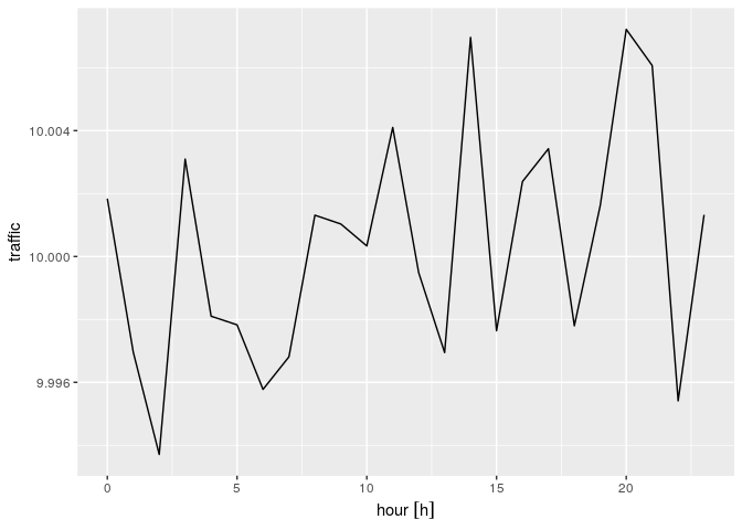
The following demonstrates how dplyr can filter bike travel, and
compute mean bike traffic by hour of day:
b <- st %>% as.tbl_cube %>%
  filter(mode == "bike") %>%
  group_by(hour) %>%
  summarise(traffic = mean(traffic)) %>%
  as.data.frame()
require(ggforce)
## Loading required package: ggforce
ggplot() +
  geom_line(data=b, aes(x=hour, y=traffic))
Raster layers and bricks
As a proof of concept, we can convert stars objects to and from raster layers (2D) or raster bricks (3D), e.g.
z.raster = as(z, "Raster")
z2 = st_as_stars(z.raster)
all.equal(z, z2, check.attributes = FALSE)
## [1] TRUE
(differences concern variable names, units, and dimension names)
Next steps
The next steps in the stars project include:
- we need to learn whether this data structure fits the needs, and is “fit” for the harder steps, involving scalability and remote computing
- develop scalable versions, where
starsobjects proxy large arrays, locally, or on a remote server - implement subset, crop, apply methods in a more generic way than
filterandsummarizenow do - create examples where we run a time-series model over each pixel
- write easy plot methods
- develop interactions with
mapview
Reactions
Reactions, questions, discussion etc. are all very welcome: either here, as issue on the project page, on twitter, or by direct email.