mapedit - interactively edit spatial data in R

• Install mapedit
• Drawing, Editing, Deleting Features
  • Proof of Concept 1 | Draw on Blank Map
  • Proof of Concept 2 | Edit and Delete Existing Features
  • Disclaimers
• Selecting Regions
  • Proof of Concept 3
• Editing Attributes
  • Proof of Concept 4
• Conclusion

[view raw Rmd]

The R ecosystem offers a powerful set of packages for geospatial analysis. For a comprehensive list see the CRAN Task View: Analysis of Spatial Data. Yet, many geospatial workflows require interactivity for smooth uninterrupted completion. With new tools, such as htmlwidgets, shiny, and crosstalk, we can now inject this useful interactivity without leaving the R environment. In the first phase of the mapedit project, we have focused on experimenting and creating proof of concepts for the following three objectives:

1. drawing, editing, and deleting features,

2. selecting and querying of features and map regions,

3. editing attributes.

Install mapedit

To run the code in the following discussion, please install with devtools::install_github. Please be aware that the current functionality is strictly a proof of concept, and the API will change rapidly and dramatically. Also mapedit's older sibling mapview will greatly enhance our abilities, so we strongly recommend installing it even though mapview is not a requirement. mapedit depends on leaflet.extras, which is currently not on CRAN, so we will also need to install it.

devtools::install_github("r-spatial/mapedit")

# although not necessary for mapedit,
#  mapview will also be very helpful, and
#  and we will use throughout this post
devtools::install_github("r-spatial/mapview")

devtools::install_github("bhaskarvk/leaflet.extras")

Drawing, Editing, Deleting Features

We would like to set up an easy process for CRUD (create, read, update, and delete) of map features. The function editMap demonstrates a first step toward this goal.

Proof of Concept 1 | Draw on Blank Map

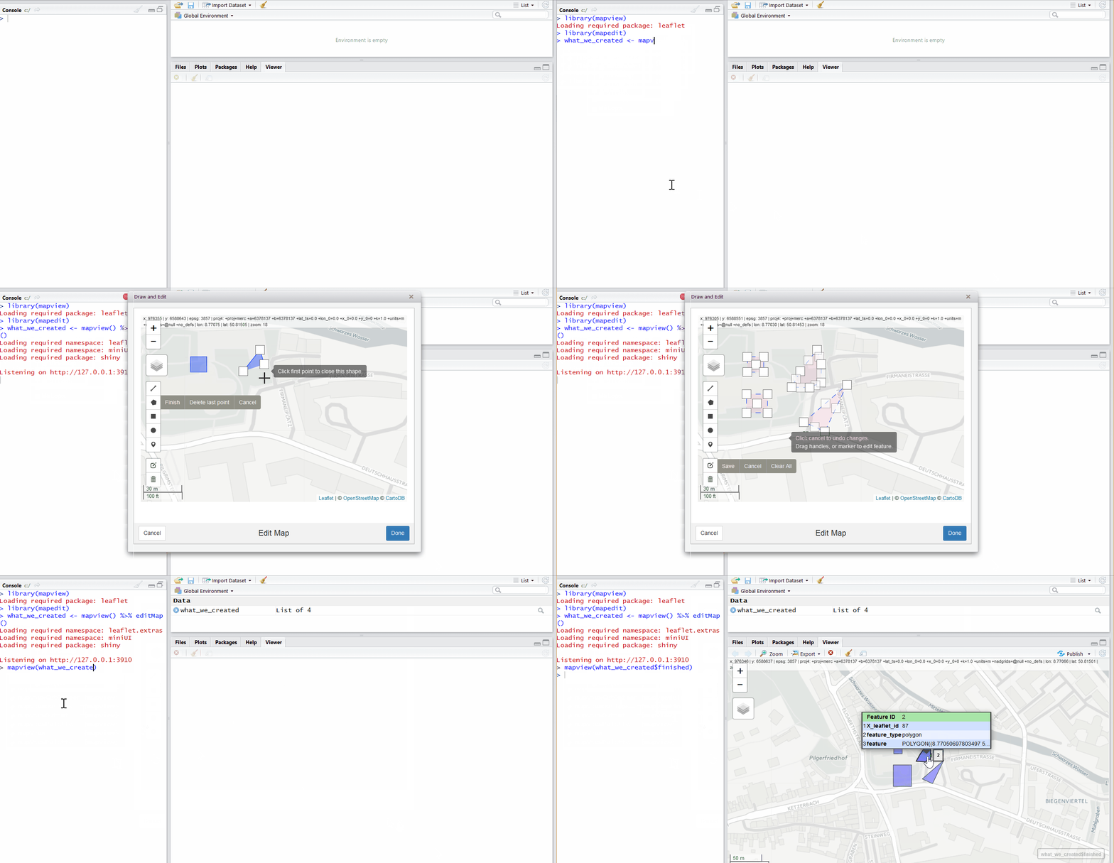
To see how we might add some features, let’s start with a blank map, and then feel free to draw, edit, and delete with the Leaflet.Draw toolbar on the map. Once finished drawing simply press “Done”.

library(mapview)
library(mapedit)

what_we_created <- mapview() %>%
  editMap()

editMap returns a list with drawn, edited, deleted, and finished features as simple features. In this case, if we would like to see our finished creation we can focus on what_we_created$finished. Since the return value is simple features, the easiest way to interactively explore what we just created will be to use mapview.

mapview(what_we_created$finished)

Proof of Concept 2 | Edit and Delete Existing Features

As an extension of the first proof of concept, we might like to edit and/or delete existing features. Let’s play Donald Trump for this exercise and use the border between Mexico and the United States for California and Arizona. For the sake of the example, let’s use a simplified polyline as our border. As we have promised we want to build a wall, but if we could just move the border a little in some places, we might be able to ease construction.

library(sf)

# simplified border for purpose of exercise
border <- st_as_sfc(
"LINESTRING(-109.050197582692 31.3535554844322, -109.050197582692 31.3535554844322, -111.071681957692 31.3723176640684, -111.071681957692 31.3723176640684, -114.807033520192 32.509681296831, -114.807033520192 32.509681296831, -114.741115551442 32.750242384668, -114.741115551442 32.750242384668, -117.158107738942 32.5652527715121, -117.158107738942 32.5652527715121)"
) %>%
  st_set_crs(4326)

# plot quickly for visual inspection
plot(border)

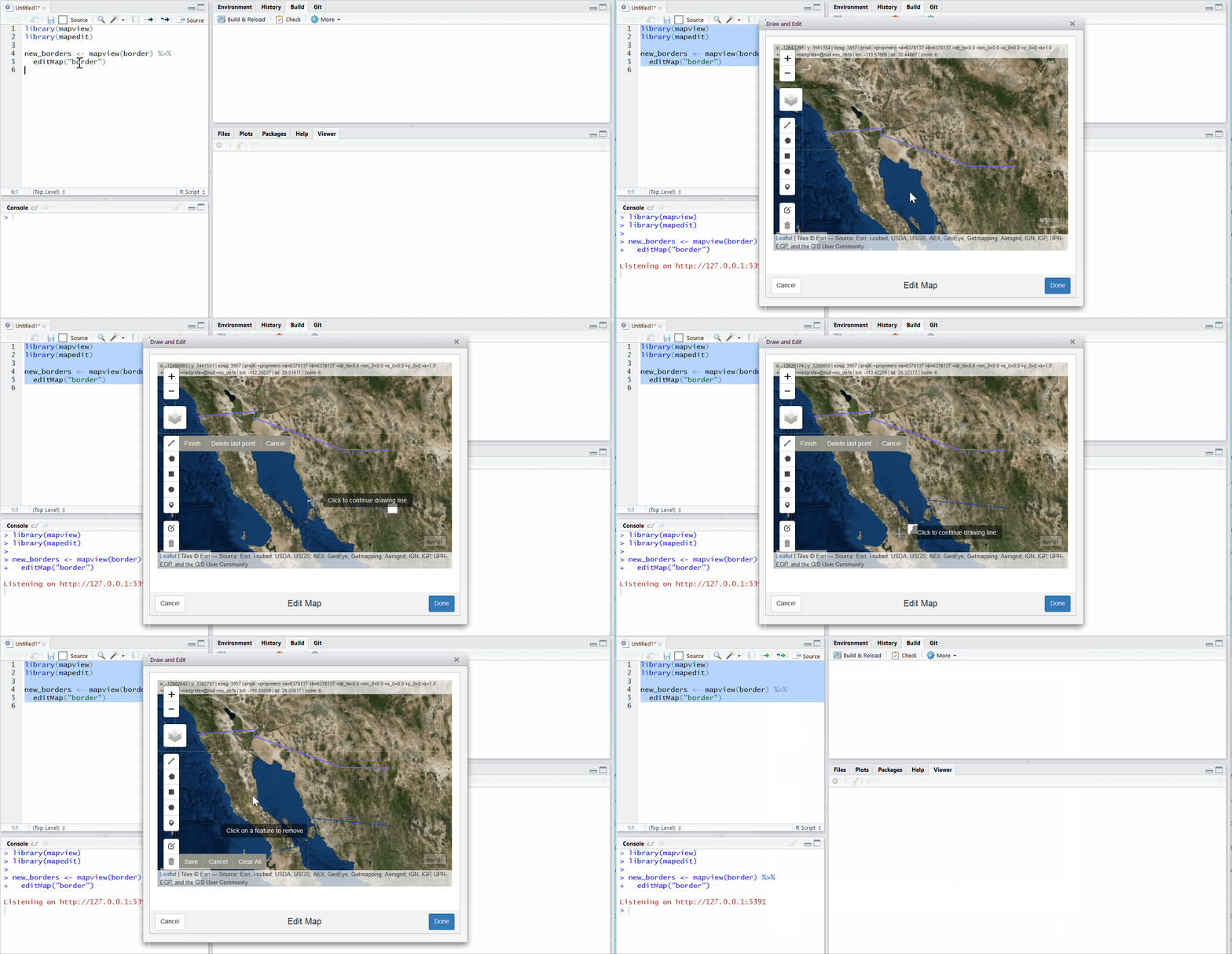
Since we are Trump, we can do what we want, so let’s edit the line to our liking. We will use mapview for our interactive map since it by default gives us an OpenTopoMap layer. With our new border and fence, we will avoid the difficult mountains and get a little extra beachfront.

library(mapview)
library(mapedit)

new_borders <- mapview(border) %>%
  editMap("border")

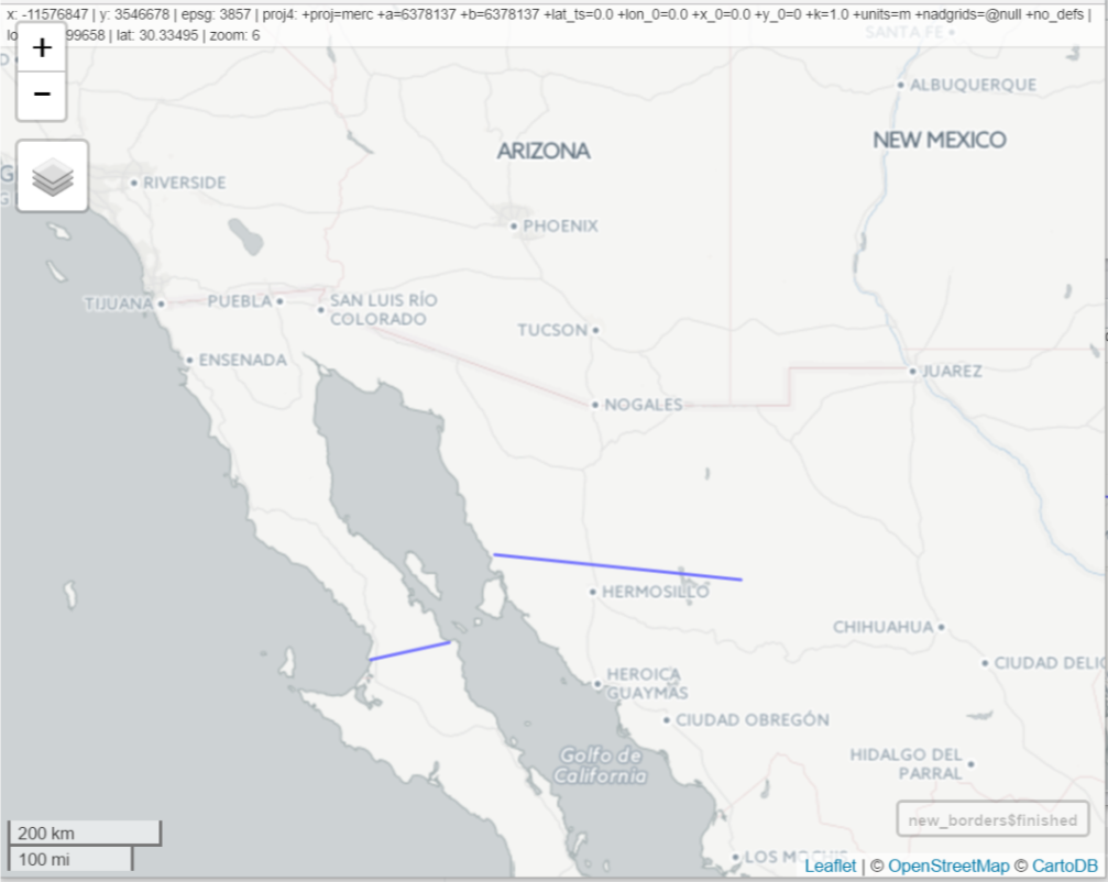
Now, we can quickly inspect our new borders and then send the coordinates to the wall construction company.

mapview(new_borders$drawn)

Disclaimers

If you played enough with the border example, you might notice a couple of glitches and missing functionality. This is a good time for a reminder that this is alpha and intended as a proof of concept. Please provide feedback, so that we can insure a quality final product. In this case, the older version of Leaflet.Draw in RStudio Viewer has some bugs, so clicking an existing point creates a new one rather than allowing editing of that point. Also, the returned list from editMap has no knowledge of the provided features.

Selecting Regions

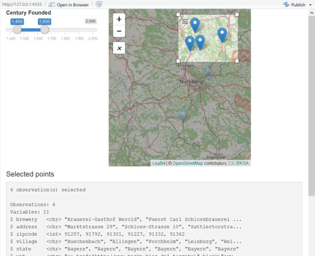
The newest version of leaflet provides crosstalk support, but support is currently limited to addCircleMarkers. This functionality is enhanced by the sf use of list columns and integration with dplyr verbs. Here is a quick example with the breweries91 data from leaflet.

library(crosstalk)
library(mapview)
library(sf)
library(shiny)
library(dplyr)

# convert breweries91 from mapview into simple features
#  and add a Century column that we will use for selection
brew_sf <- st_as_sf(breweries91) %>%
  mutate(century = floor(founded/100)*100) %>%
  filter(!is.na(century)) %>%
  mutate(id=1:n())

pts <- SharedData$new(brew_sf, key = ~id, group = "grp1")

ui <- fluidPage(
  fluidRow(
    column(4, filter_slider(id="filterselect", label="Century Founded", sharedData=pts, column=~century, step=50)),
    column(6, leafletOutput("leaflet1"))
  ),
  h4("Selected points"),
  verbatimTextOutput("selectedpoints")
)

server <- function(input, output, session) {
  # unfortunatly create SharedData again for scope
  pts <- SharedData$new(brew_sf, key = ~id, group = "grp1")
  lf <- leaflet(pts) %>%
    addTiles() %>%
    addMarkers()
  
  not_rendered <- TRUE
  # hack to only draw leaflet once
  output$leaflet1 <- renderLeaflet({
    if(req(not_rendered,cancelOutput=TRUE)) {
      not_rendered <- FALSE
      lf
    }
  })
  
  output$selectedpoints <- renderPrint({
    df <- pts$data(withSelection = TRUE)
    cat(nrow(df), "observation(s) selected\n\n")
    str(dplyr::glimpse(df))
  })
}

shinyApp(ui, server)

With mapedit, we would like to enhance the geospatial crosstalk integration to extend beyond leaflet::addCircleMarkers. In addition, we would like to provide an interactive interface to the geometric operations of sf, such as st_intersects(), st_difference(), and st_contains().

Proof of Concept 3

As a select/query proof of concept, assume we want to interactively select some US states for additional analysis. We will build off Bhaskar Karambelkar’s leaflet projection example using Bob Rudis albersusa package.

# use @bhaskarvk USA Albers with leaflet code
#  https://bhaskarvk.github.io/leaflet/examples/proj4Leaflet.html
#devtools::install_github("hrbrmstr/albersusa")
library(albersusa)
library(sf)
library(leaflet)
library(mapedit)

spdf <- usa_composite() %>% st_as_sf()
pal <- colorNumeric(
  palette = "Blues",
  domain = spdf$pop_2014
)

bounds <- c(-125, 24 ,-75, 45)

(lf <- leaflet(
  options=
    leafletOptions(
      worldCopyJump = FALSE,
      crs=leafletCRS(
        crsClass="L.Proj.CRS",
        code='EPSG:2163',
        proj4def='+proj=laea +lat_0=45 +lon_0=-100 +x_0=0 +y_0=0 +a=6370997 +b=6370997 +units=m +no_defs',
        resolutions = c(65536, 32768, 16384, 8192, 4096, 2048,1024, 512, 256, 128)
      ))) %>%
  fitBounds(bounds[1], bounds[2], bounds[3], bounds[4]) %>%
  setMaxBounds(bounds[1], bounds[2], bounds[3], bounds[4]) %>%
  mapview::addFeatures(
    data=spdf, weight = 1, color = "#000000",
    # adding group necessary for identification
    layerId = ~iso_3166_2,
    fillColor=~pal(pop_2014),
    fillOpacity=0.7,
    label=~stringr::str_c(name,' ', format(pop_2014, big.mark=",")),
    labelOptions= labelOptions(direction = 'auto')#,
    #highlightOptions = highlightOptions(
    #  color='#00ff00', bringToFront = TRUE, sendToBack = TRUE)
  )
)


# test out selectMap with albers example
selectMap(
  lf,
  styleFalse = list(weight = 1),
  styleTrue = list(weight = 4)
)

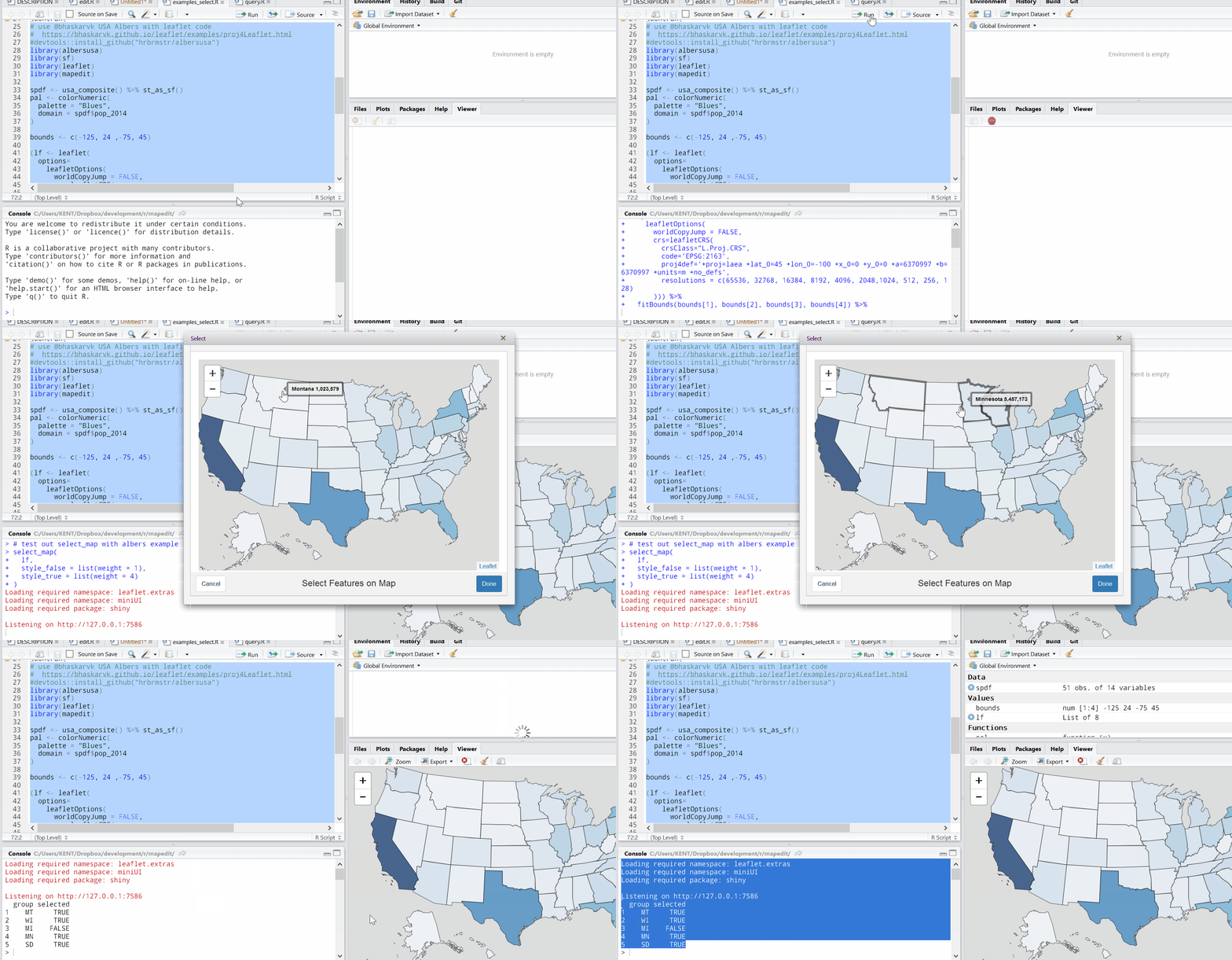
The selectMap() function will return a data.frame with an id/group column and a selected column. selectMap() will work with nearly all leaflet overlays and offers the ability to customize the styling of selected and unselected features.

Editing Attributes

A common task in geospatial analysis involves editing or adding feature attributes. While much of this can be accomplished in the R console, an interactive UI on a reference map can often help perform this task. Mapbox’s geojson.io provides a good reference point for some of the features we would like to provide in mapedit.

Proof of Concept 4

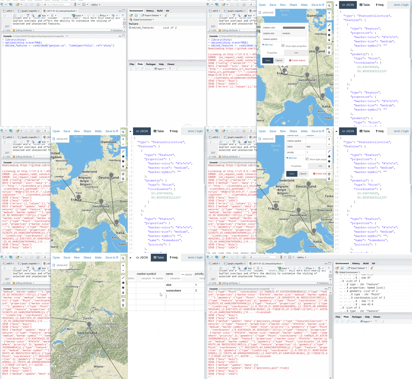
As a proof of concept, we made a Shiny app that thinly wraps a slightly modified geojson.io. Currently, we will have to pretend that there is a mechanism to load R feature data onto the map, since this functionality does not yet exist.

library(shiny)
edited_features <- runGitHub(
  "geojson.io", "timelyportfolio", ref="shiny"
)

Conclusion

mapedit hopes to add useful interactivity to your geospatial workflows by leveraging powerful new functionality in R with the interactivity of HTML, JavaScript, and CSS. mapedit will be better with your feedback, requests, bug reports, use cases, and participation. We will report on progress periodically with blog posts on this site, and we will develop openly on the mapedit Github repo.