MNF/MAF, PCA, and EOFs of time series, spatial and spatio-temporal data
Introduction
The Maximum Noise Fraction (MNF, Green et al., 1988) transform tries to split a multivariate signal into a factors that have an increasing signal-to-noise ratio. The model it underlies is that the covariance of a signal \(Z\), \(\Sigma\), can be decomposed into two independent covariance components,
\[\Sigma = \Sigma_N + \Sigma_S.\]
MNF factors are obtained by projecting the data on the eigenvectors of \(\Sigma_N \Sigma_S^{-1}\). The challenge is to obtain \(\Sigma_N\). One way is by computing the covariance of the first order differences, assuming the noise is temporally uncorrelated. This way, the MNF transform is identical to Min/Max Autocorrelation Factors (MAFs, Switzer and Green, 1984).
Time Series: noise in one band
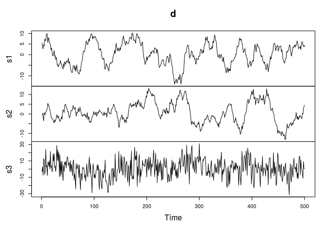
When noise it is unevenly distributed over the bands, MNF isolates the noise in its first band(s). We create three identical, temporally correlated signals, and add (a lot of) noise to the third:
set.seed(13531) # reproducible
s1 = arima.sim(list(ma = rep(1,20)), 500)
s2 = arima.sim(list(ma = rep(1,20)), 500)
s3 = arima.sim(list(ma = rep(1,20)), 500)
s3 = s3 + rnorm(500, sd = 10)
d = cbind(s1,s2,s3)
plot(d)
Next, we can compute the MNF transform using the mnf method in package
spacetime 1.2-0, devel,
library(spacetime)
m = mnf(d)
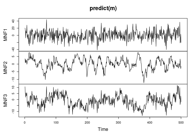
plot(predict(m))
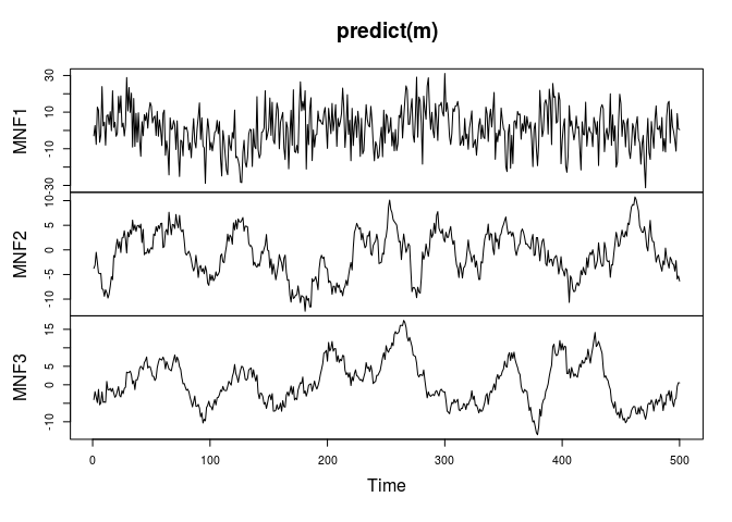
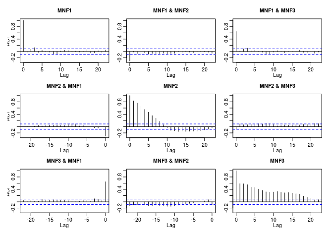
which reveals that the first MNF component (MAF) captures the noise, the remaining two the signals. The autocorrelation functions of the MNF components confirms this:
acf(predict(m))
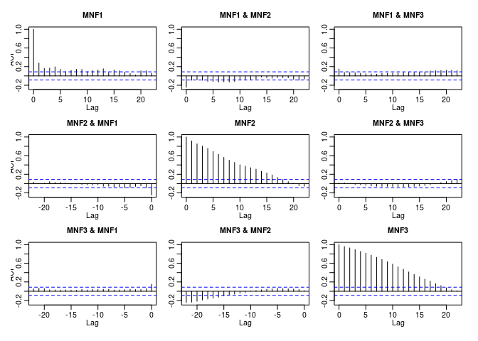
and also confirms that the last component has the strongest autocorrelation.
Interpretation of eigenvalues
class(m)

## [1] "mnf"    "prcomp"

m$values

## [1] 0.72449579 0.05187041 0.03045926

m

## Standard deviations:
## [1] 0.8511732 0.2277508 0.1745258
##
## Rotation:
##              [,1]        [,2]        [,3]
## [1,] -0.001939465 -0.76418567 -0.65807011
## [2,] -0.012781443 -0.63770953  0.74957909
## [3,]  0.999916433 -0.09667895  0.07123842

summary(m)

## Importance of components:
##                          [,1]    [,2]    [,3]
## Standard deviation     0.8512 0.22775 0.17453
## Proportion of Variance 0.8980 0.06429 0.03775
## Cumulative Proportion  0.8980 0.96225 1.00000
In contrast to both Switzer and Green (1984) and Green et al. (1988) we used \(0.5 Cov(Z(x)-Z(x+\Delta))\) to estimate \(\Sigma_N\), rather than \(Cov(Z(x)-Z(x+\Delta))\). This does not affect the eigenvectors, but ensures that eigenvalues stay between 0 and 1, where under the proportional covariance model they have the more natural interpretation as approximate estimators of the noise fraction for each component. One minus the value is the lag one autocorrelation of the corresponding component.
The Cumulative Proportion suggests that the first component takes care
of 90% of the noise, the first two of 96% of the noise. MAF Components
are ordered by decreasing noise fraction.
Time Series: correlated noise in multiple bands
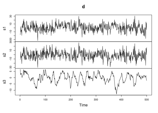
When noise it is unevenly distributed over the bands, MNF isolates the noise in its first band(s). We create three identical, temporally correlated signals, and add (a lot of) noise to the third. We see that all noise is captured in the first MNF component, and consequent components have increasing autocorrelation:
n1 = rnorm(500, sd = 10)
s1 = arima.sim(list(ma = rep(1,20)), 500) + n1
s2 = arima.sim(list(ma = rep(0.5,20)), 500) + n1
s3 = arima.sim(list(ma = rep(1,10)), 500)
d = cbind(s1,s2,s3)
plot(d)
m = mnf(d)
m$values

## [1] 1.02487353 0.08970645 0.06573597

plot(predict(m))
acf(predict(m))
Principal Components on the same series
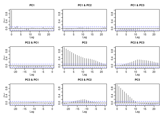
PCA does a very differnt thing: it also captures the (correlated) noise signal in component 1, but does not rank the following components according to increasing autocorrelation:
acf(predict(prcomp(d)))
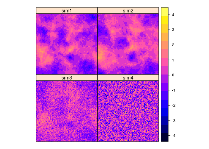
Spatial data
We generate four fields with strong spatial correlation and strong cross correlation, and noise in one band:
library(sp)
grd = SpatialPoints(expand.grid(x=1:100, y=1:100))
gridded(grd) = TRUE
fullgrid(grd) = TRUE
pts = spsample(grd, 50, "random")
pts$z = rnorm(50)
library(gstat)
v = vgm(1, "Sph", 90)
out = krige(z~1, pts, grd, v, nmax = 20, nsim = 4)

## drawing 4 GLS realisations of beta...
## [using conditional Gaussian simulation]

out[[3]] = 0.5 * out[[3]] + 0.5 * rnorm(1e4)
out[[4]] = rnorm(1e4)
spplot(out, as.table = TRUE)
Then, MNFs are obtained by
m = mnf(out)
m

## Standard deviations:
## [1] 0.9987070 0.9043657 0.3433185 0.1704122
##
## Rotation:
##               [,1]        [,2]        [,3]        [,4]
## [1,] -0.0008221442 -0.01481666 -0.74522878 -0.64549885
## [2,] -0.0013281490 -0.01466196  0.66638999 -0.69030983
## [3,]  0.0469361062  0.98542516 -0.01412851 -0.32651402
## [4,]  0.9988966724 -0.16882759 -0.01894281 -0.01386252

summary(m)

## Importance of components:
##                          [,1]   [,2]    [,3]   [,4]
## Standard deviation     0.9987 0.9044 0.34332 0.1704
## Proportion of Variance 0.5083 0.4168 0.06007 0.0148
## Cumulative Proportion  0.5083 0.9251 0.98520 1.0000
and can be plotted by
spplot(predict(m), as.table = TRUE)
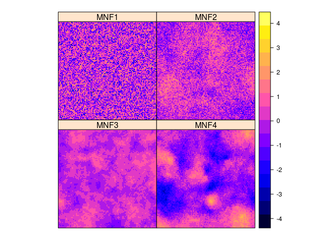
We see that MNF4 is an inversion of the signal in sim1 and sim2.
The variograms of the MNFs show a clear increase in spatial correlation,
from MNF1 to MNF4.
pr = predict(m)
g = gstat(NULL, "MNF1", MNF1~1, pr)
g = gstat(g,    "MNF2", MNF2~1, pr)
g = gstat(g,    "MNF3", MNF3~1, pr)
g = gstat(g,    "MNF4", MNF4~1, pr)
#plot(variogram(g))
The following methods have been implemented for mnf in spacetime:
methods(mnf)

## [1] mnf.matrix*                 mnf.mts*
## [3] mnf.RasterBrick*            mnf.RasterStack*
## [5] mnf.SpatialGridDataFrame*   mnf.SpatialPixelsDataFrame*
## [7] mnf.zoo*
## see '?methods' for accessing help and source code
EOFs
Empirical Orthogonal Functions are eigenvectors for spatio-temporal
data. An example of there use is found in section 7.4 of the spacetime
vignette.
References
- Green, A.A., Berman, M., Switzer, P. and Craig, M.D., 1988. A transformation for ordering multispectral data in terms of image quality with implications for noise removal. Geoscience and Remote Sensing, IEEE Transactions on, 26(1), pp.65-74.
- Switzer, P. and Green, A., 1984. Min/max autocorrelation factors for multivariate spatial imagery: Dept. of Statistics. Stanford University, Tech. Rep. 6.