Spatial indexes give you fast results on spatial queries, such as finding whether pairs of geometries intersect or touch, or finding their intersection. They reduce the time to get results from quadratic in the number of geometries to linear in the number of geometries. A recent commit brings spatial indexes to sf for the binary logical predicates (intersects, touches, crosses, within, contains, contains_properly, overlaps, covers, covered_by, relate_pattern, equals, disjoint), as well as intersection, which returns intersecting geometries.

The spatial join function st_join uses a logical predicate to join features, and is also also affected by this speedup.

Antecedents

There have been attempts to use spatial planar indices, including enhancement issue sfr:76. In rgeos, GEOS STRtrees were used in rgeos/src/rgeos_poly2nb.c, which is mirrored in a modern Rcpp setting sf/src/geos.cpp, around lines 276 and 551. The STRtree is constructed by building envelopes (bounding boxes) of input entities, which are then queried for intersection with envelopes of another set of entities (in rgeos, R functions gUnarySTRtreeQuery and gBinarySTRtreeQuery). The use case was to find neighbours of all the about 90,000 US Census entities in Los Angeles, via spdep::poly2nb(), which received an argument to enter the candidate neighbours found by Unary querying the STRtree of entities by the same entities.

Benchmark

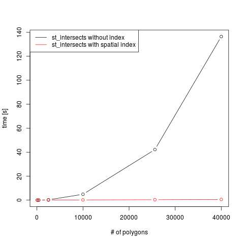
A simple benchmark shows the obvious: st_intersects without spatial index behaves quadratic in the number of geometries (black line), and is much faster for the case where a spatial index is created, stronger so for larger number of polygons:

The polygon datasets used are simple checker boards with square polygons (showing a nice Moiré pattern):

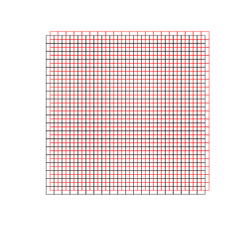
The black small square polygons are essentially matched to the red ones; the number of polygons along the x axis is the number of a single geometry set (black).

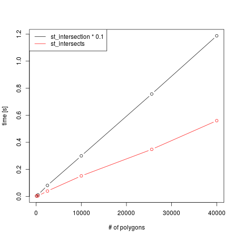
To show that the behaviour of intersects and intersection is indeed linear in the number of polygons, we show runtimes for both, as a function of the number of polygons (where intersection was divided by 10 for scaling purposes):

Implementation

Spatial indexes are available in the GEOS library used by sf, through the functions starting with STRtree. The algorithm implements a Sort-Tile-Recursive R-tree, according to the JTS documentation described in P. Rigaux, Michel Scholl and Agnes Voisard. Spatial Databases With Application To GIS. Morgan Kaufmann, San Francisco, 2002.

The sf implementation (some commits to follow this one) excludes some binary operations. st_distance, and st_relate without pattern, are excluded as these need to go through all combinations, returning a dense matrix. st_equals_exact is excluded as approximate matches are sought, without constraining the degree of approximation.

On which argument is an index built?

The R-tree is built on the first argument (x), and used to match all geometries over the second argument (y) of binary functions. This could give runtime differences, but for instance for the dataset that triggered this development in sfr:394, we see hardly any difference:

library(sf)
# Linking to GEOS 3.5.1, GDAL 2.1.3, proj.4 4.9.2, lwgeom 2.3.2 r15302
load("test_intersection.Rdata")
nrow(test)
# [1] 16398
nrow(hsg2)
# [1] 6869
system.time(int1 <- st_intersection(test, hsg2))
#    user  system elapsed 
# 105.712   0.040 105.758 
system.time(int2 <- st_intersection(hsg2, test))
#    user  system elapsed 
# 107.756   0.060 107.822 
# Warning messages:
# 1: attribute variables are assumed to be spatially constant throughout all geometries 
# 2: attribute variables are assumed to be spatially constant throughout all geometries 

The resulting feature sets int1 and int2 are identical, only the order of the features (records) and of the attribute columns (variables) differs. Runtime without index is 35 minutes, 20 times as long.

Is the spatial index always built?

In the current implemenation (version >= 0.5-1) the index is always built, except for st_distance, and st_relate without pattern. This means it is also built e.g. for rook or queen neighborhood selections (sfr:234), which use st_relate with a specified pattern.

What about prepared geometries?

Prepared geometries in GEOS are essentially indexes over single geometries and not over sets of geometries; they speed things up in particular when single geometries are very complex, and only for a single geometry to single geometry comparison. The spatial indexes are indexes over collections of geometries; they make a cheap preselection based on bounding boxes before the expensive pairwise comparison takes place.

Script used

The followinig script was used to create the benchmark plots. It no longer works; in the version where it worked, prepared = FALSE would take a branch where no trees were built, this is no longer the case.

 library(sf)
 sizes = c(10, 20, 50, 100, 160, 200)
 res = matrix(NA, length(sizes), 4)
 for (i in seq_along(sizes)) {
     g1 = st_make_grid(st_polygon(list(rbind(c(0,0),c(0,1),c(1,1),c(0,1),c(0,0)))), n = sizes[i]) * sizes[i]
     g2 = g1 + c(.5,.5)
     res[i, 1] = system.time(i1 <- st_intersects(g1, g2))[1]
     res[i, 2] = system.time(i2 <- st_intersects(g1, g2, prepare = FALSE))[1]
     res[i, 3] = system.time(i1 <- st_intersection(g1, g2))[1]
     res[i, 4] = identical(i1, i2)
 }
 plot(sizes^2, res[,2], type = 'b', ylab = 'time [s]', xlab = '# of polygons')
 lines(sizes^2, res[,1], type = 'b', col = 'red')
 legend("topleft", lty = c(1,1), col = c(1,2), legend = c("st_intersects without index", "st_intersects with spatial index"))
 plot(sizes^2, res[,3]/10, type = 'b', ylab = 'time [s]', xlab = '# of polygons')
 lines(sizes^2, res[,1], type = 'b', col = 'red')
 legend("topleft", lty = c(1,1), col = c(1,2), legend = c("st_intersection * 0.1", "st_intersects"))