sf - plot, graticule, transform, units, cast, is
- Direct linking to Proj.4
- plotting
- graticules
- geosphere and units support
- type casting
- type selection
This year began with the R Consortium blog on simple features:
#rstats A new post by Edzer Pebesma reviews the status of the R Consortium’s Simple Features project: https://t.co/W8YqH3WQVJ
— Joseph Rickert (@RStudioJoe) January 3, 2017
This blog post describes changes of sf 0.2-8 and upcoming 0.2-9, compared to 0.2-7, in more detail.
Direct linking to Proj.4
Since 0.2-8, sf links directly to the Proj.4 library:
library(sf)

## Linking to GEOS 3.5.0, GDAL 2.1.0, proj.4 4.9.2
before that, it would use the projection interface of GDAL, which uses
Proj.4, but exposes only parts of it. The main reason for switching to
Proj.4 is the ability for stronger error checking. For instance, where
GDAL would interpret any unrecognized field for +datum as WGS84:
# sf 0.2-7:
> st_crs("+proj=longlat +datum=NAD26")
$epsg
[1] NA

$proj4string
[1] "+proj=longlat +ellps=WGS84 +no_defs"

attr(,"class")
[1] "crs"
Now, with sf 0.2-8 we get a proper error in case of an unrecognized
+datum field:
t = try(st_crs("+proj=longlat +datum=NAD26"))
attr(t, "condition")

## <simpleError in make_crs(x): invalid crs: +proj=longlat +datum=NAD26, reason: unknown elliptical parameter name>
plotting
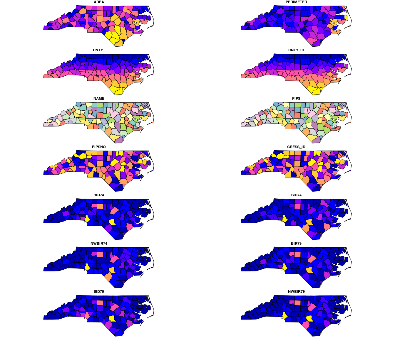
The default plot method for sf objects (simple features with
attributes, or data.frames with a simple feature geometry list-column)
now plots the set of maps, one for each attribute, with automatic color
scales:
nc = st_read(system.file("gpkg/nc.gpkg", package="sf"), quiet = TRUE)
plot(nc)
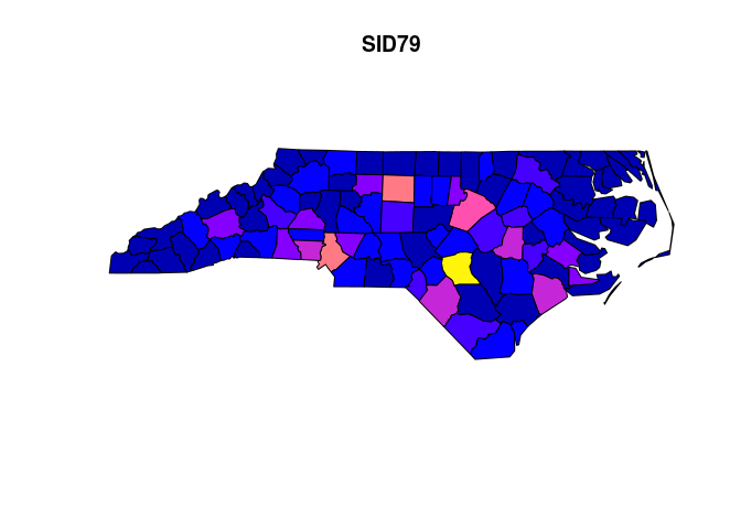
well, that is all there is, basically. For plotting a single map, select the appropriate attribute
plot(nc["SID79"])
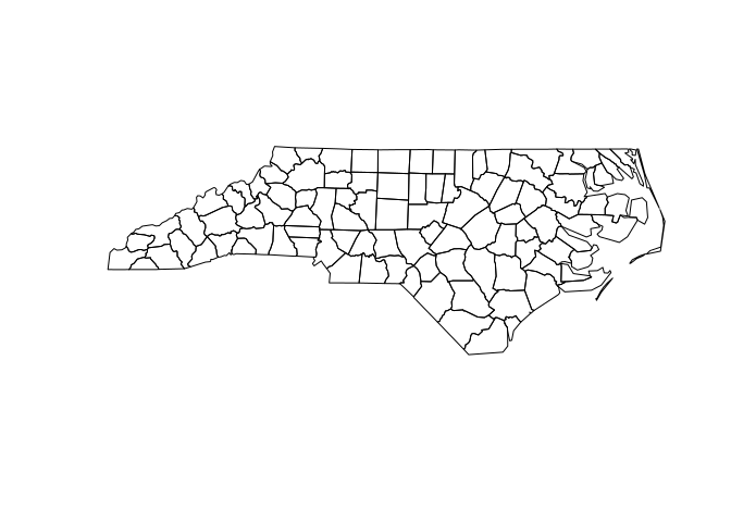
or only the geometry:
plot(st_geometry(nc))
graticules
Package sf gained a function st_graticule to generate graticules,
grids formed by lines with constant longitude or latitude. Suppose we
want to project nc to the state plane, and plot it with a longitude
latitude graticule in NAD27 (the original datum of nc):
nc_sp = st_transform(nc["SID79"], 32119) # NC state plane, m
plot(nc_sp, graticule = st_crs(nc), axes = TRUE)

The underlying function, st_graticule, can be used directly to
generate a simple object with graticules, but is rather meant to be used
by plotting functions that benefit from a graticule in the background,
such as plot or ggplot. The function provides the end points of
graticules and the angle at which they end; an example for using Lambert
equal area on the USA is found in the help page of st_graticule:
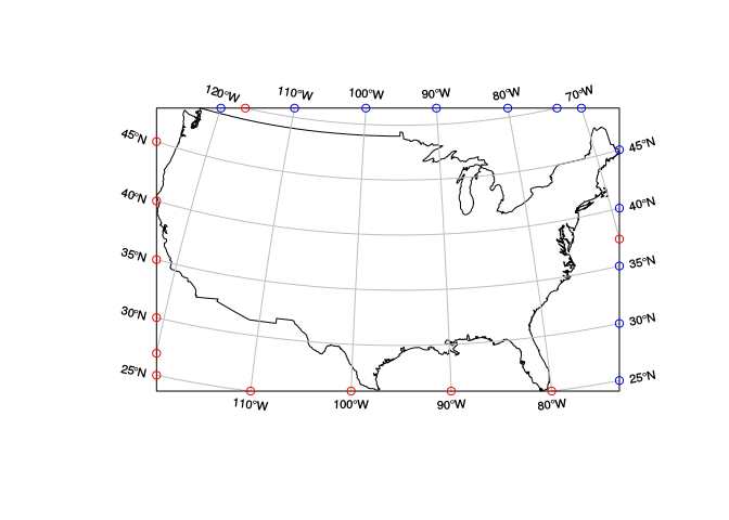
The default plotting method for simple features with longitude/latitude
coordinates is the equirectangular
projection,
(also called geographic projection, or equidistant cylindrical (eqc)
projection) which linearly maps longitude and latitude into \(x\) and
\(y\), transforming \(y\) such that in the center of the map 1 km
easting equals 1 km northing. This is also the default for sp::plot,
sp::spplot and ggplot2::coord_quickmap. The official Proj.4
transformation for this is found
here.
We can obtain e.g. a plate carrée projection (with one degree latitude equaling one degree longitude) with
caree = st_crs("+proj=eqc")
plot(st_transform(nc[1], caree), graticule = st_crs(nc), axes=TRUE, lon = -84:-76)
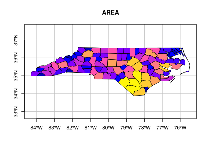
and we see indeed that the lon/lat grid is formed of squares.
The usual R plot for nc obtained by
plot(nc[1], graticule = st_crs(nc), axes = TRUE)

corrects for latitude. The equivalent, officially projected map is
obtained by using the eqc projection with the correct latitude:
mean(st_bbox(nc)[c(2,4)])

## [1] 35.23582

eqc = st_crs("+proj=eqc +lat_ts=35.24")
plot(st_transform(nc[1], eqc), graticule = st_crs(nc), axes=TRUE)
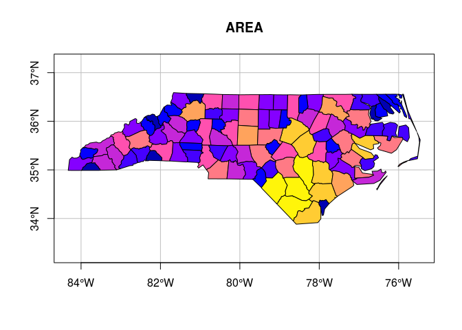
so that in the center of these (identical) maps, 1 km east equals 1 km north.
geosphere and units support
sf now uses functions in package
geosphere to compute
distances or areas on the sphere. This is only possible for points and
not for arbitrary feature geometries:
centr = st_centroid(nc)

## Warning in st_centroid.sfc(st_geometry(x)): st_centroid does not give
## correct centroids for longitude/latitude data

st_distance(centr[c(1,10)])[1,2]

## 34093.21 m
As a comparison, we can compute distances in two similar projections, each having a different measurement unit:
centr.sp = st_transform(centr, 32119) # NC state plane, m
(m <- st_distance(centr.sp[c(1,10)])[1,2])

## 34097.54 m

centr.ft = st_transform(centr,  2264) # NC state plane, US feet
(ft <- st_distance(centr.ft[c(1,10)])[1,2])

## 111868.3 US_survey_foot
and we see that the units are reported, by using package units. To verify that the distances are equivalent, we can compute
ft/m

## 1 1
which does automatic unit conversion before computing the ratio. (Here,
1 1 should be read as one, unitless (with unit 1)).
For spherical distances, sf uses geosphere::distGeo. It passes on
the parameters of the datum, as can be seen from
st_distance(centr[c(1,10)])[1,2]                     # NAD27

## 34093.21 m

st_distance(st_transform(centr, 4326)[c(1,10)])[1,2] # WGS84

## 34094.28 m
Other measures come with units too, e.g. st_area
st_area(nc[1:5,])

## Units: m^2
## [1] 1137388604  611077263 1423489919  694546292 1520740530
units vectors can be coerced to numeric by
as.numeric(st_area(nc[1:5,]))

## [1] 1137388604  611077263 1423489919  694546292 1520740530
type casting
With help from Mike Sumner and Etienne Racine, we managed to get a
working st_cast, which helps converting one geometry in another.
casting individual geometries (sfg)
Casting individual geometries will close polygons when needed:
st_point(c(0,1)) %>% st_cast("MULTIPOINT")

## MULTIPOINT(0 1)

st_linestring(rbind(c(0,1), c(5,6))) %>% st_cast("MULTILINESTRING")

## MULTILINESTRING((0 1, 5 6))

st_linestring(rbind(c(0,0), c(1,0), c(1,1))) %>% st_cast("POLYGON")

## POLYGON((0 0, 1 0, 1 1, 0 0))
and will warn on loss of information:
st_linestring(rbind(c(0,1), c(5,6))) %>% st_cast("POINT")

## Warning in st_cast.LINESTRING(., "POINT"): point from first coordinate only

## POINT(0 1)

st_multilinestring(list(matrix(1:4,2), matrix(1:6,,2))) %>% st_cast("LINESTRING")

## Warning in st_cast.MULTILINESTRING(., "LINESTRING"): keeping first
## linestring only

## LINESTRING(1 3, 2 4)
casting sets of geometries (sfc)
Casting sfc objects can group or ungroup geometries:
# group:
st_sfc(st_point(0:1), st_point(2:3), st_point(4:5)) %>%
    st_cast("MULTIPOINT", ids = c(1,1,2))

## Geometry set for 2 features
## geometry type:  MULTIPOINT
## dimension:      XY
## bbox:           xmin: 0 ymin: 1 xmax: 4 ymax: 5
## epsg (SRID):    NA
## proj4string:    NA

## MULTIPOINT(0 1, 2 3)

## MULTIPOINT(4 5)

# ungroup:
st_sfc(st_multipoint(matrix(1:4,,2))) %>% st_cast("POINT")

## Geometry set for 2 features
## geometry type:  POINT
## dimension:      XY
## bbox:           xmin: 1 ymin: 3 xmax: 2 ymax: 4
## epsg (SRID):    NA
## proj4string:    NA

## POINT(1 3)

## POINT(2 4)
st_cast with no to argument will convert mixes of GEOM and
MULTIGEOM to MULTIGEOM, where GEOM is POINT, LINESTRING or
POLYGON, e.g.
st_sfc(
    st_multilinestring(list(matrix(5:8,,2))),
    st_linestring(matrix(1:4,2))
  ) %>% st_cast()

## Geometry set for 2 features
## geometry type:  MULTILINESTRING
## dimension:      XY
## bbox:           xmin: 1 ymin: 3 xmax: 6 ymax: 8
## epsg (SRID):    NA
## proj4string:    NA

## MULTILINESTRING((5 7, 6 8))

## MULTILINESTRING((1 3, 2 4))
or unpack geometry collections:
x <- st_sfc(
    st_multilinestring(list(matrix(5:8,,2))),
    st_point(c(2,3))
  ) %>% st_cast("GEOMETRYCOLLECTION")
x

## Geometry set for 2 features
## geometry type:  GEOMETRYCOLLECTION
## dimension:      XY
## bbox:           xmin: 2 ymin: 3 xmax: 6 ymax: 8
## epsg (SRID):    NA
## proj4string:    NA

## GEOMETRYCOLLECTION(MULTILINESTRING((5 7, 6 8)))

## GEOMETRYCOLLECTION(POINT(2 3))

x %>% st_cast()

## Geometry set for 2 features
## geometry type:  GEOMETRY
## dimension:      XY
## bbox:           xmin: 2 ymin: 3 xmax: 6 ymax: 8
## epsg (SRID):    NA
## proj4string:    NA

## MULTILINESTRING((5 7, 6 8))

## POINT(2 3)
casting on sf objects
The casting of sf objects works in principle identical, except that
for ungrouping, attributes are repeated (and might give rise to warning
messages),
# ungroup:
st_sf(a = 1, geom = st_sfc(st_multipoint(matrix(1:4,,2)))) %>%
    st_cast("POINT")

## Warning in st_cast.sf(., "POINT"): repeating attributes for all sub-
## geometries for which they may not be constant

## Simple feature collection with 2 features and 1 field
## geometry type:  POINT
## dimension:      XY
## bbox:           xmin: 1 ymin: 3 xmax: 2 ymax: 4
## epsg (SRID):    NA
## proj4string:    NA
##   c.1..1.       geom
## 1       1 POINT(1 3)
## 2       1 POINT(2 4)
and for grouping, attributes are aggregated, which requires an aggregation function
# group:
st_sf(a = 1:3, geom = st_sfc(st_point(0:1), st_point(2:3), st_point(4:5))) %>%
    st_cast("MULTIPOINT", ids = c(1,1,2), FUN = mean)

## Simple feature collection with 2 features and 2 fields
## geometry type:  MULTIPOINT
## dimension:      XY
## bbox:           xmin: 0 ymin: 1 xmax: 4 ymax: 5
## epsg (SRID):    NA
## proj4string:    NA
##   ids.group   a                 geom
## 1         1 1.5 MULTIPOINT(0 1, 2 3)
## 2         2   3      MULTIPOINT(4 5)
type selection
In case we have a mix of geometry types, we can select those of a
particular geometry type by the new helper function st_is. As an
example we create a mix of polygons, lines and points:
g = st_makegrid(n=c(2,2), offset = c(0,0), cellsize = c(2,2))
s = st_sfc(st_polygon(list(rbind(c(1,1), c(2,1),c(2,2),c(1,2),c(1,1)))))
i = st_intersection(st_sf(a=1:4, geom = g), st_sf(b = 2, geom = s))

## Warning in st_intersection(st_sf(a = 1:4, geom = g), st_sf(b = 2, geom =
## s)): attribute variables are assumed to be spatially constant throughout
## all geometries

i

## Simple feature collection with 4 features and 2 fields
## geometry type:  GEOMETRY
## dimension:      XY
## bbox:           xmin: 1 ymin: 1 xmax: 2 ymax: 2
## epsg (SRID):    NA
## proj4string:    NA
##   a b                       geometry
## 1 1 2 POLYGON((2 2, 2 1, 1 1, 1 2...
## 2 2 2           LINESTRING(2 2, 2 1)
## 3 3 2           LINESTRING(1 2, 2 2)
## 4 4 2                     POINT(2 2)
and can select using dplyr::filter, or directly using st_is:
filter(i, st_is(geometry, c("POINT")))

## Simple feature collection with 1 feature and 2 fields
## geometry type:  GEOMETRY
## dimension:      XY
## bbox:           xmin: 1 ymin: 1 xmax: 2 ymax: 2
## epsg (SRID):    NA
## proj4string:    NA
##   a b   geometry
## 1 4 2 POINT(2 2)

filter(i, st_is(geometry, c("POINT", "LINESTRING")))

## Simple feature collection with 3 features and 2 fields
## geometry type:  GEOMETRY
## dimension:      XY
## bbox:           xmin: 1 ymin: 1 xmax: 2 ymax: 2
## epsg (SRID):    NA
## proj4string:    NA
##   a b             geometry
## 1 2 2 LINESTRING(2 2, 2 1)
## 2 3 2 LINESTRING(1 2, 2 2)
## 3 4 2           POINT(2 2)

st_is(i, c("POINT", "LINESTRING"))

## [1] FALSE  TRUE  TRUE  TRUE